
ACU-T: 6108 AcuSolve - EDEM Bidirectional Coupling with User-Defined Drag Model
Tutorial Level: Advanced
Prerequisites
This tutorial covers the setup process for running a bidirectional AcuSolve EDEM coupled simulation using a custom user-defined drag model. An overview of the UDF code and the compilation process is provided in the beginning of the tutorial, followed by the simulation setup and post-processing. It is assumed that you have prior experience using HyperMesh CFD and EDEM, the basics of which are covered in the tutorials: ACU-T: 1000 UI Introduction, and ACU-T: 6100 Particle Separation in a Windshifter using Altair EDEM .
Problem Description
The problem to be solved is shown schematically in the figure below. In this tutorial, you will learn how to write a custom UDF for calculating the drag force on a solid particle in a creeping flow also known as Stokes flow. In Stokes flow, the fluid velocities are generally significantly low, or the fluid viscosities are significantly high and are characterized by very low particle Reynolds numbers (<<1) indicating that the inertial forces are negligible compared to the viscous forces. Stokes flow can be observed in microfluidic devices, blood flow in capillaries, solid particle sedimentation in quiescent fluid, and so on. According to the Stokes drag law, the total drag force (pressure drag plus shear stress drag) on a particle is given by:
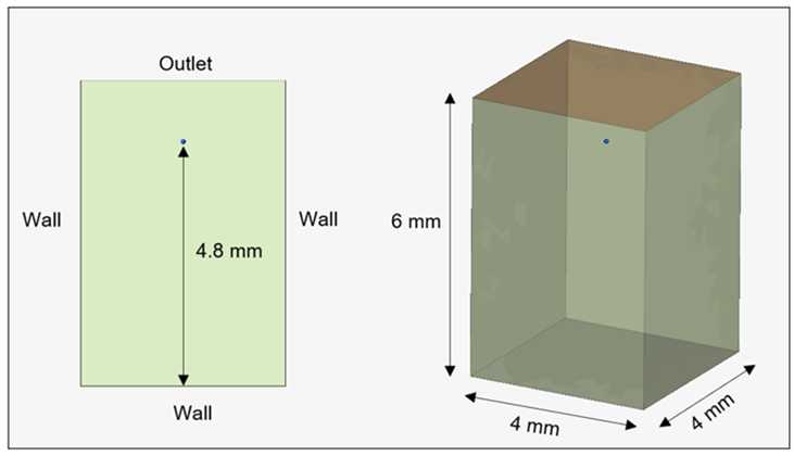
The objective of the simulation is to calculate the terminal velocity of the solid particle as it falls through the water column. The particle’s initial location is 4.8 mm from the bottom of the water column. Under Stokes flow, the particle initially accelerates due to gravity and the fluid drag force is negligible. As the particle moves through the fluid, the frictional drag increases and the acceleration reduces to zero over time and thereafter the particle travels with a constant velocity, known as the terminal velocity.
| Important Simulation Parameters | |
|---|---|
| Water density (kg/m3) | 1000 |
| Water viscosity (Pa s) | 0.001 |
| Particle density (kg/m3) | 1500 |
| Particle diameter (m) | 0.0001 |
AcuSolve User-Defined Function (UDF) Overview
UDF Format
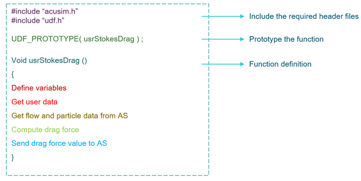
Header Files
- acusim.h: This header file includes the main data types
used by AcuSolve and the standard C header files
such as stdio.h, string.h and
math.h. Common data types used by AcuSolve:
a. Integer Type integer b. Real Type floating point c. String Type string d. Void Type void - udf.h: This header file contains all of the macros and declarations needed for accessing the data in the UDF.
Function Prototype
Once the header files are declared, you need to prototype the user function using the UDF_PROTOTYPE() macro and the name of the user function as the argument. For example, UDF_PROTOTYPE(usrStokesDrag).
This user function name should be the same as the one specified in the model setup. Otherwise, it can lead to run time errors. Although the user function names can be anything that is supported by C, it is good practice to use function names that start with usr to distinguish the user functions from other solver parameters.
Function Definition
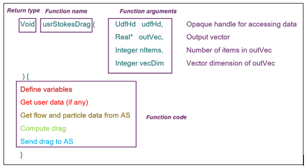
Return Type
All C functions should have a return type. Since the drag force values should be sent back to AcuSolve through outVec, the return value does not have any significance and the return type should be set to Void.
Function Arguments
- udfHd
- Pointer which contains the necessary information for accessing various data. All supporting routines require this argument.
- outVec
- Resulting vector of the user function. On input this array contains all zeros. This vector is used to send the force information back to AcuSolve.
- nItems
- This is the first dimension of outVec, which specifies the number of items that needs to be filled. For all drag model user functions, the value is 1 since you are calculating the drag force on 1 particle in each call.
- vecDim
- This is the second dimension of outVec which specifies the vector dimension of the particular data. This value depends on the type of data that is sent back.
- Drag user function
- Minimum three values (x, y ,z components) are required. Optionally a fourth value can also be sent back to AcuSolve (drag coefficient).
- Lift user function
- Three values (x, y, z components).
- Torque user function
- Three values (x, y, z components).
Function Code
Variables:
Variables are used to store certain types of data. This data can be a single value or an array of values. In C language, all variables need to be declared before they can be used in the program. Although the declaration can be done anywhere inside the program, declaring all the required variables upfront makes the code more organized and easily understandable. The syntax for declaring a variable in C is Datatype variable_name ;
Example
Real volume ;
where Real is the data type and volume is the name of the variable.
In many UDFs, including the current example, you may need to access some data from AcuSolve which has already been calculated and stored by the solver at a particular memory address. For this, you need to declare pointer variables which point to the memory address of the requested data. For instance, if you need to access the local fluid velocity, you need to declare a pointer variable that stores the memory address of the location where AcuSolve has already stored the value.
Example
Real* xVel ;
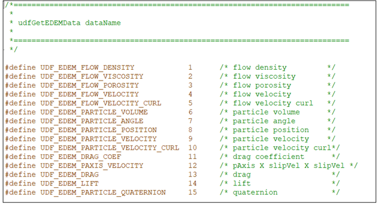
Accessing data from AcuSolve:
The routine to be used for accessing particle and fluid data from AcuSolve is udfGetEDEMData(udfHd, dataName). This returns an array of data and length of the array depends on the type of data that is requested.
For example,
To access the particle’s volume, first you need to declare a pointer variable and then use the following data routine.
Real* vol ;
- Calculate drag force values:
- Send force data to AcuSolve:
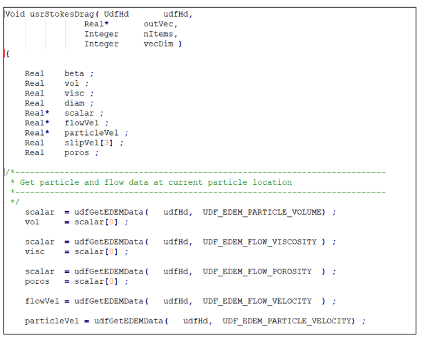
Full Code Snippet
#include "acusim.h"
#include "udf.h"
/*===========================================================================
*
* Prototype the function
*
*===========================================================================
*/
UDF_PROTOTYPE( usrStokesDrag ) ;
/*===========================================================================
*
* "stokesDrag": calculate EDEM particle drag force based on the Stokes law
*
* Arguments:
* udfHd - opaque handle for accessing information
* outVec - output vector
* nItems - number of items in outVec (=1 in this case)
* vecDim - vector dimension of outVec (=3 in this case)
*
* Input file parameters:
* user_values = { }
* user_strings = { "" }
*
*===========================================================================
*/
Void usrStokesDrag( UdfHd udfHd,
Real* outVec,
Integer nItems,
Integer vecDim )
{
Real beta ;
Real vol ;
Real visc ;
Real diam ;
Real* scalar ;
Real* flowVel ;
Real* particleVel ;
Real slipVel[3] ;
Real poros ;
/*---------------------------------------------------------------------------
* Get particle and flow data at current particle location
*---------------------------------------------------------------------------
*/
scalar = udfGetEDEMData( udfHd, UDF_EDEM_PARTICLE_VOLUME) ;
vol = scalar[0] ;
scalar = udfGetEDEMData( udfHd, UDF_EDEM_FLOW_VISCOSITY ) ;
visc = scalar[0] ;
scalar = udfGetEDEMData( udfHd, UDF_EDEM_FLOW_POROSITY ) ;
poros = scalar[0] ;
flowVel = udfGetEDEMData( udfHd, UDF_EDEM_FLOW_VELOCITY ) ;
particleVel = udfGetEDEMData( udfHd, UDF_EDEM_PARTICLE_VELOCITY) ;
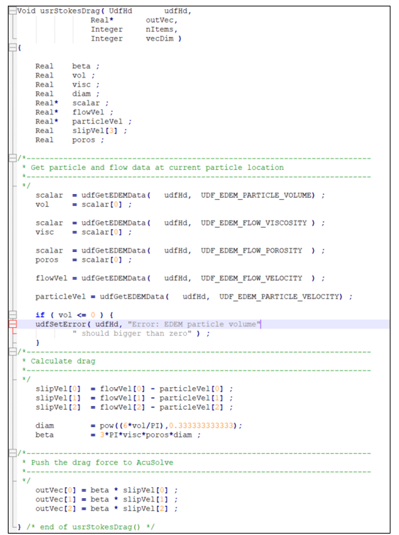
if ( vol <= 0 ) {
udfSetError( udfHd, "Error: EDEM particle volume"
" should bigger than zero" ) ;
}
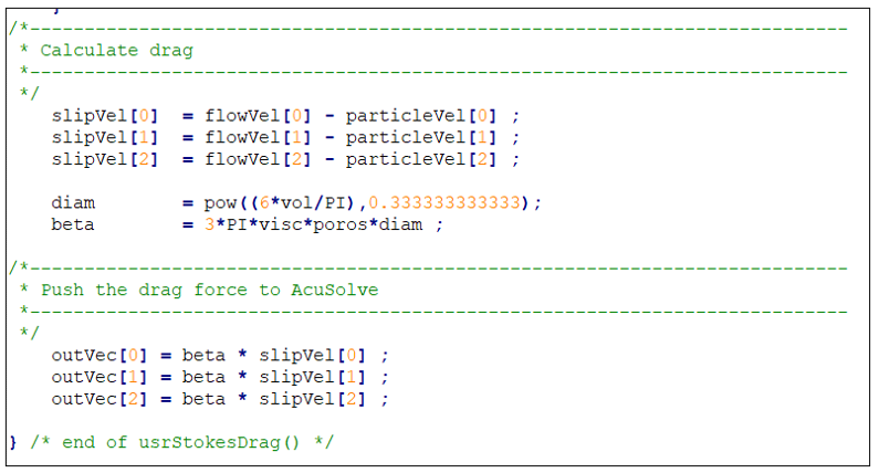
/*---------------------------------------------------------------------------
* Calculate drag
*---------------------------------------------------------------------------
*/
slipVel[0] = flowVel[0] - particleVel[0] ;
slipVel[1] = flowVel[1] - particleVel[1] ;
slipVel[2] = flowVel[2] - particleVel[2] ;
diam = pow((6*vol/PI),0.333333333333);
beta = 3*PI*visc*poros*diam ;
/*---------------------------------------------------------------------------
* Push the drag force to AcuSolve
*---------------------------------------------------------------------------
*/
outVec[0] = beta * slipVel[0] ;
outVec[1] = beta * slipVel[1] ;
outVec[2] = beta * slipVel[2] ;
} /* end of usrStokesDrag() */For more information about the UDF routines available refer to the AcuSolve User-Defined Functions Manual.
Compiling the UDF
For the solver to access the user-defined functions, the functions must be compiled and linked into a shared library. These libraries should be placed in the problem directory along with the solver input files.
Windows
From the Start menu, expand Altair <solver version> and launch the AcuSolve Cmd Prompt.
In the terminal, cd to the directory where the model files and the UDF script file are located. Then execute the following command to compile the UDF:
acuMakeDll -src usrStokesDrag.c
Linux
Open a command line prompt and cd to the directory where the model files and the UDF script are located. Then execute the following command:
acuMakeLib -src usrStokesDrag.c
Part 1 – AcuSolve Simulation
Start HyperMesh CFD and Open the HyperMesh Database
- Start HyperMesh CFD from the Windows Start menu by clicking .
-
From the Home tools, Files tool group, click the Open Model tool.
Figure 7. 
The Open File dialog opens. -
Browse to the directory where you saved the model file. Select the HyperMesh file ACU-T6108_sphere.hm and click Open.
This will be the working directory and all of the files related to the simulation will be stored in this location.
Validate the Geometry
The Validate tool scans through the entire model, performs checks on the surfaces and solids, and flags any defects in the geometry, such as free edges, closed shells, intersections, duplicates, and slivers.
Set Up Flow
Set the General Simulation Parameters
-
From the Flow ribbon, click the Physics tool.
Figure 9. 
The Setup dialog opens. - Under the Physics models setting, select the Multiphase flow radio button.
- Change the Multifluid type to Bidirectional EDEM Coupling.
-
Click the Eulerian material drop-down menu and select Material
Library from the list.
You can create new material models in the Material Library.
-
In the Material Library dialog, select EDEM 2 Way
Multiphase, switch to the My Material
tab, and then click
 to add a new material model.
- In the microdialog, click EDEM Bidirectional Material in the top-left corner and change the name to Water-Particle.
- Set the Carrier field to Water.
- Verify that the Particle Shape is set to Spherical and set the Drag model to User Function.
-
Click the table icon beside the drag model drop-down.
Figure 10. 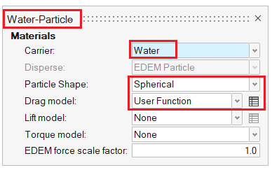
-
In the new dialog, set the Function name to
usrStokesDrag.
Note: The function name entered here should be the same as the name of the UDF_PROTOTPYE in the UDF. The user-function name can be any name supported in C that starts with the letters usr.
Figure 11. 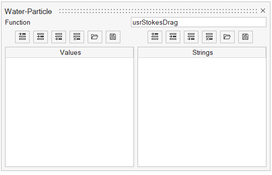
- Press Esc to close the dialog.
- Close the Material Model and Material Library dialogs.
- In the Setup dialog, set the Eulerian material to Water-Particle.
- Set Time step size and Final time to 5e-05 and 0.015, respectively.
-
Set the Turbulence model to Laminar.
The calculated particle Reynolds number is less than 0.3 which is in the Stokes regime where the viscous forces dominate the inertial forces and the turbulence effects can be neglected.
- Verify that Gravity is set to 0, 0, -9.81.
-
Set the Pressure scale to Absolute.
Figure 12. 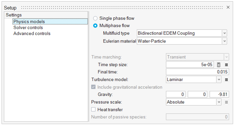
-
Click the Solver controls setting and set the
Minimum/Maximum stagger iterations to 2,
respectively.
Figure 13. 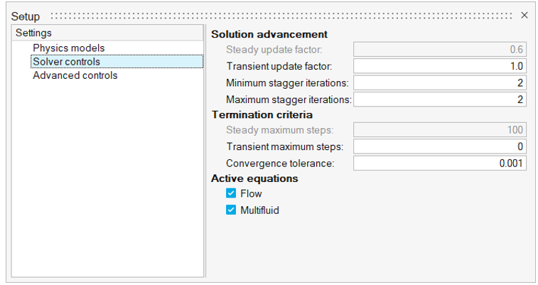
- Close the dialog and save the model.
Assign Material Properties
-
From the Flow ribbon, click the Material tool.
Figure 14. 
-
Verify that Water-Particle has been assigned as the material.
If not assigned, click the geometry and select Water-Particle from the microdialog.
-
On the guide bar, click
 to exit
the tool.
to exit
the tool.
Define Flow Boundary Conditions
-
Click the Outlet tool in the
Boundaries group.
Figure 15. 
-
In the modeling window, click the top surface of the
model, which is highlighted in the figure below.
Figure 16. 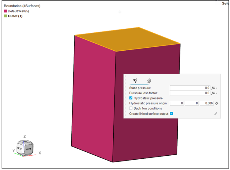
- In the microdialog, activate the Hydrostatic pressure option and set the Hydrostatic pressure origin to (0, 0, 0.006.)
-
Click on the guide bar.
Note: A no-slip wall condition is assigned to all surfaces by default.
- Save the model.
Generate the Mesh
-
From the Mesh ribbon, click the
Volume tool.
Figure 17. 
The Meshing Operations dialog opens. - In the Meshing Operations dialog, set the Mesh size to Average Size and set the Average element size to 0.0005.
- Deactivate Curvature-based surface refinement and then click Mesh.
Define Nodal Outputs
Once the meshing is complete, you are automatically taken to the Solution ribbon.
-
From the Solution ribbon, click the Field tool.
Figure 18. 
The Field Output dialog opens. - Check the box for Write initial conditions.
- Check the box for Write results at time step interval.
-
Set the Time step interval to 5.
Figure 19. 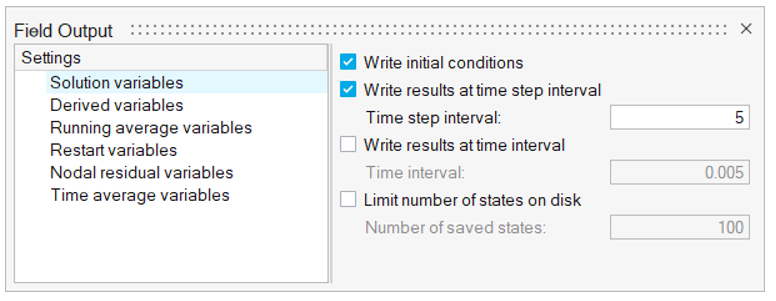
- Close the dialog and save the model.
Part 2 - EDEM Simulation
Start Altair EDEM from the Windows start menu by clicking .
Open the EDEM Input Deck
- In the Creator tab in EDEM, go to .
-
Browse to the directory where you saved the sphere.dem
file and open it.
This loads the geometry and the materials.
Figure 20. 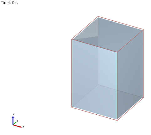
Review the EDEM Model Setup
The main area of focus for this tutorial is the user-defined drag model setup and compilation process for a bidirectional AcuSolve - EDEM coupling simulation. Therefore, for the sake of brevity, the EDEM database provided with the input files contains all of the required setup.
Summary of the EDEM Model
A spherical particle of diameter 0.0001 m is introduced in a water column at a point which is 0.0048 m from the bottom. Since the density of the particle is 1500 kg/m3, that is, heavier than water, the particle falls freely through the water column.
Define the Simulation Settings
-
Click
 in the top-left corner to go to
the EDEM Simulator tab.
in the top-left corner to go to
the EDEM Simulator tab.
- In the Simulator Settings tab, set the Time Integration scheme to Euler and deactivate the Auto Time Step checkbox.
-
Enter a value of 1e-6s for Fixed Time Step.
Note: Generally, a value of 20-40% of the Rayleigh Time Step is recommended as the time step size to ensure stability of the DEM simulation. Since the DEM time steps are usually a few orders lower than the CFD time step, for every CFD time step the DEM solver performs multiple iterations to match with the CFD time. Therefore, the CFD time step should always be an integer multiple of DEM time step to ensure that the physical times in both AcuSolve and EDEM match.
- Set the Total Time to 0.015 s and the Target Save Interval to 0.00015 s.
- Set the Cell Size to 2.5 R min.
-
Set the Selected Engine to CPU Solver and set the Number
of CPU Cores based on availability.
Figure 21. 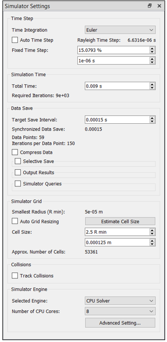
- Once the simulation settings have been defined, save the model.
Submit the Coupled Simulation
-
Start the coupling server by clicking Coupling Server in
EDEM.
Figure 22. 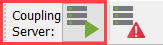
Once the Coupling server is activated, the icon changes.Figure 23. 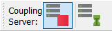
- Return to HyperMesh CFD.
-
From the Solution ribbon, click the Run tool.
Figure 24. 
The Launch AcuSolve dialog opens. - Set the Parallel processing option to Intel MPI.
- Set the Number of processors to 6.
- Uncheck Automatically define pressure reference.
- Expand Default initial conditions, uncheck Pre-compute flow and set the velocity values to 0. Uncheck Pre-compute Turbulence.
-
Click Run to launch AcuSolve.
Figure 25. 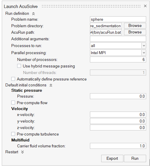
Once the AcuSolve run is launched, the Run Status dialog opens.
-
In the dialog, right-click the AcuSolve run and
select View log file.
If the coupling with EDEM is successful, that information is printed in the .log file.
Figure 26. 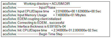
Once the simulation is complete, the summary of the run time is printed at the end of the .log file.
Analyze the Results
-
Once the EDEM simulation is complete, click
 in the top-left corner to go to
the EDEM Analyst tab.
in the top-left corner to go to
the EDEM Analyst tab.
-
Click the Create Graph icon.
Figure 27. 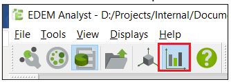
-
In the Analyst tree, select the Line plot and make sure
that the parameters for X-axis are set as shown in the figure below.
Figure 28. 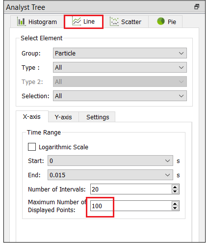
- Click the Y-axis tab and set the Primary Attribute to Velocity and the Component to Magnitude (Average).
-
Click Create Graph.
Figure 29. 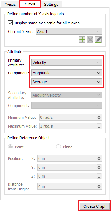
The particle velocity vs time plot displays in the plot window.Figure 30. 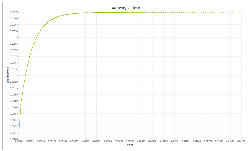
As expected, at the beginning of the simulation, the particle accelerates from zero-velocity because of gravity. As the particle moves and displaces the surrounding fluid, the frictional drag on the particle increases and due to the combined effect of buoyancy and drag force, the acceleration reduces to 0 and the particle moves with a constant velocity. This is known as the particle terminal velocity and in this case the predicted value is 0.00274 m/s which is very close (0.5% error) to the analytical solution (0.002725 m/s). This shows that the Stokes drag law is very accurate in predicting the fluid-induced drag forces for creeping flows.
Summary
In this tutorial, you learned how to write a user-defined function in C programming language for implementing a custom drag model for bidirectional AcuSolve-EDEM coupling. The Stokes drag law was used to calculate the terminal velocity of a spherical particle falling through a water column. The simulation results showed that the Stokes drag law is quite accurate in predicting the drag force on a particle in low Reynolds number flows.