
ACU-T: 6000 Static Mixer Simulation – AcuTrace
Tutorial Level: Intermediate
Prerequisites
This tutorial provides the instructions for setting up, solving and viewing results for a simulation of a static mixer in combination with the post-processing module AcuTrace. In this simulation, AcuSolve is used to compute the species mixing within a simple mixer and AcuTrace is used to compute the particle motion of finite mass particles within the mixer. This tutorial is designed to introduce you to concepts necessary to visualize particulate flow with AcuTrace.
- Generation of finite mass particle with AcuTrace.
- Conversion of the nodal output data with AcuTransTrace for reading into HyperMesh CFD Post.
- Post-processing the nodal output with HyperMesh CFD Post to visualize particles movement.
Problem Description
The problem to be addressed in this tutorial is shown schematically in Figure 1. It consists of a mixing tube that contains several swept walls to instigate mixing within the tube. The diameter of the inlet is 0.1 m and the length of the mixing tube is 0.525 m. The fins have a mean diameter of 0.1 m. The maximum thickness of the fins is 0.003 m.

The boundary condition at the inlet is defined to produce a fully developed inlet profile with velocity of 1.0 m/s. One portion of the inlet is defined to contain 100 percent of species_1, while the other inlet is defined to contain 0.0 percent of species_1.
The fluid in this problem is an epoxy resin, which has a density of 1264.0 kg/m3 and a viscosity of 1.49 kg/m-sec.
Start HyperMesh CFD and Open the HyperMesh Database
- Start HyperMesh CFD from the Windows Start menu by clicking .
-
From the Home tools, Files tool group, click the Open Model tool.
Figure 2. 
The Open File dialog opens. - Browse to the directory where you saved the model file. Select the HyperMesh file ACU-T6000_Static_Mixer.hm and click Open.
- Click .
-
Create a new directory named Static_Mixer and navigate into this directory.
This will be the working directory and all the files related to the simulation will be stored in this location.
- Enter Static_Mixer as the file name for the database, or choose any name of your preference.
- Click Save to create the database.
Validate the Geometry
The Validate tool scans through the entire model, performs checks on the surfaces and solids, and flags any defects in the geometry, such as free edges, closed shells, intersections, duplicates, and slivers.
Set Up the Problem
Set Up the Simulation Parameters and Solver Settings
-
From the Flow ribbon, click the Physics tool.
Figure 4. 
The Setup dialog opens. -
Under the Physics models setting:
- Verify that the Time marching is set to Steady.
- Select Spalart-Allmaras as the Turbulence model.
- Set the Number of passive species to 1.
Figure 5. 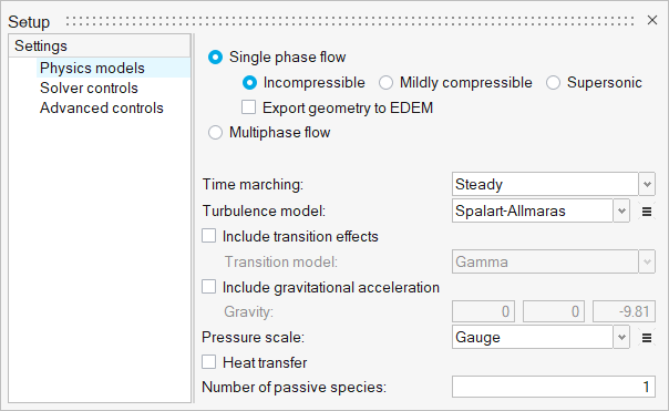
-
Click the Solver controls setting and verify that the
parameters are set as shown in the figure below.
Figure 6. 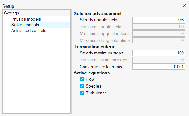
- Close the dialog and save the model.
Define the Material Model
-
From the Flow ribbon, click the Material Library tool.
Figure 7. 
The Material Library dialog opens. - Click the My Materials tab.
-
Click
 to add a new fluid material model.
- In the material creation dialog, click the name in the top-left corner and rename the material to Epoxy Resin.
-
In the Density tab:
- Set the Type to Constant.
- Set the Density value to 1264 kg/m3.
- Set the Isothermal compressibility value to 0.
Figure 8. 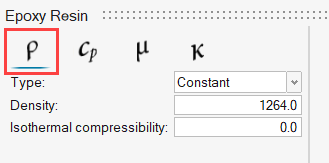
-
Click the Specific Heat tab and set the Specific heat
value to 2386 J/kg-K.
Figure 9. 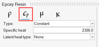
-
Click the Viscosity tab and set the Viscosity value to
1.49 kg/m-s.
Figure 10. 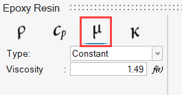
-
Click the Conductivity tab and set the Conductivity
value to 0.286 W/m-K and Turbulent Prandtl number to
0.91.
Figure 11. 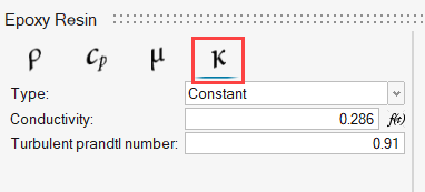
- Close all dialogs and save the model.
Assign Material Properties
-
From the Flow ribbon, click the Material tool.
Figure 12. 
-
Select the solid model and then select Epoxy_Resin as
the fluid medium.
Figure 13. 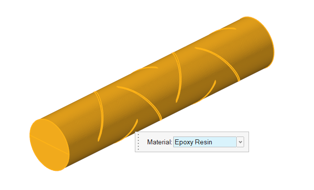
-
On the guide bar, click
 to execute
the command and exit the tool.
to execute
the command and exit the tool.
Define Flow Boundary Conditions
-
From the Flow ribbon, Profiled
tool group, click the Profiled Inlet tool.
Figure 14. 
-
In the modeling window, click the inlet surface
highlighted in the figure below.
Figure 15. 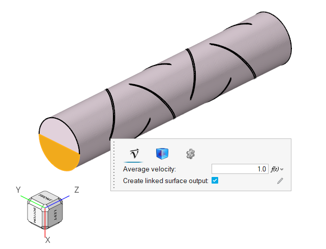
- In the microdialog, set the Average velocity to 1.0 m/s.
-
Click the Species tab and enter a value of
1.0 for Species 1.
Figure 16. 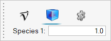
-
On the guide bar, click
 to execute the command and remain in the
tool.
to execute the command and remain in the
tool.
- Right-click Inlet in the Boundaries legend and select Rename. Change the name to Inlet S1.
-
Select the other inlet surface highlighted in the figure below.
Figure 17. 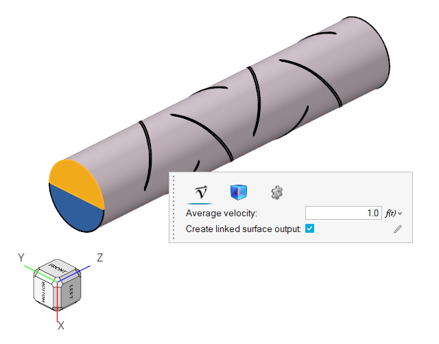
- In the microdialog, set the Average velocity to 1.0 m/s.
- Click the Species tab and enter a value of 0.0 for Species 1.
-
On the guide bar, click
to execute the command and remain in the
tool.
- Right-click Inlet in the Boundaries legend and select Rename. Change the name to Inlet S2.
-
Click the Outlet tool.
Figure 18. 
-
Select the surface highlighted below and then click
 on the guide bar.
Figure 19. 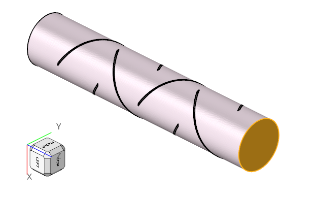
-
Click the No Slip tool.
Figure 20. 
-
Select the wall of the tube highlighted in the figure below and then click
on the guide bar.
Figure 21. 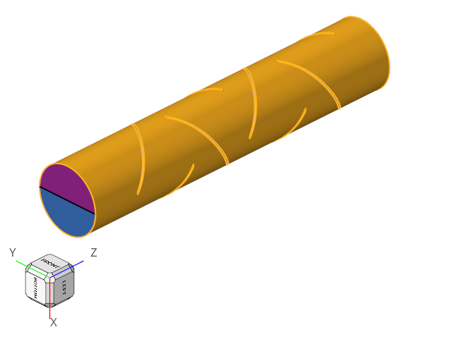
- Rename the surface group from Wall to Pipe Wall.
- Right-click Default Wall in the Boundaries legend and select Isolate.
-
Select all the surfaces highlighted in the figure below and then click
on the guide bar.
Figure 22. 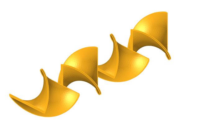
- Rename the surface group from Wall to Fin Walls.
-
Click
 on the guide bar.
- Turn on the visibility of all the surfaces by right-clicking in the modeling window and selecting Show All or by simply pressing the A key.
- Save the model.
Define Surface Monitors and Run AcuSolve
-
From the Solution ribbon, click the Volumes tool.
Figure 23. 
-
Select the model and then click
on the guide bar.
Figure 24. 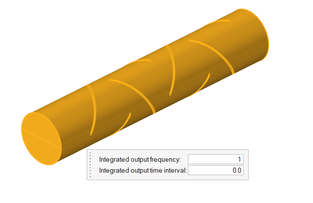
-
Click on the guide bar.
-
From the Solution ribbon, click the Run tool.
Figure 25. 
The Launch AcuSolve dialog opens. - Make sure the problem directory is set to the correct location. If not, use the Browse option to select the correct directory.
- Set the Parallel processing option to Intel MPI.
- Optional: Set the number of processors to 4 or 8 based on availability.
-
Leave the remaining default options and then click Run
to launch AcuSolve.
Figure 26. 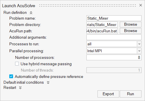
Post-Process With the Plot Tool
-
From the Solution ribbon, click the Plot tool.
Figure 27. 
-
Observe the residual and solution ratios as the simulation progresses.
Figure 28. 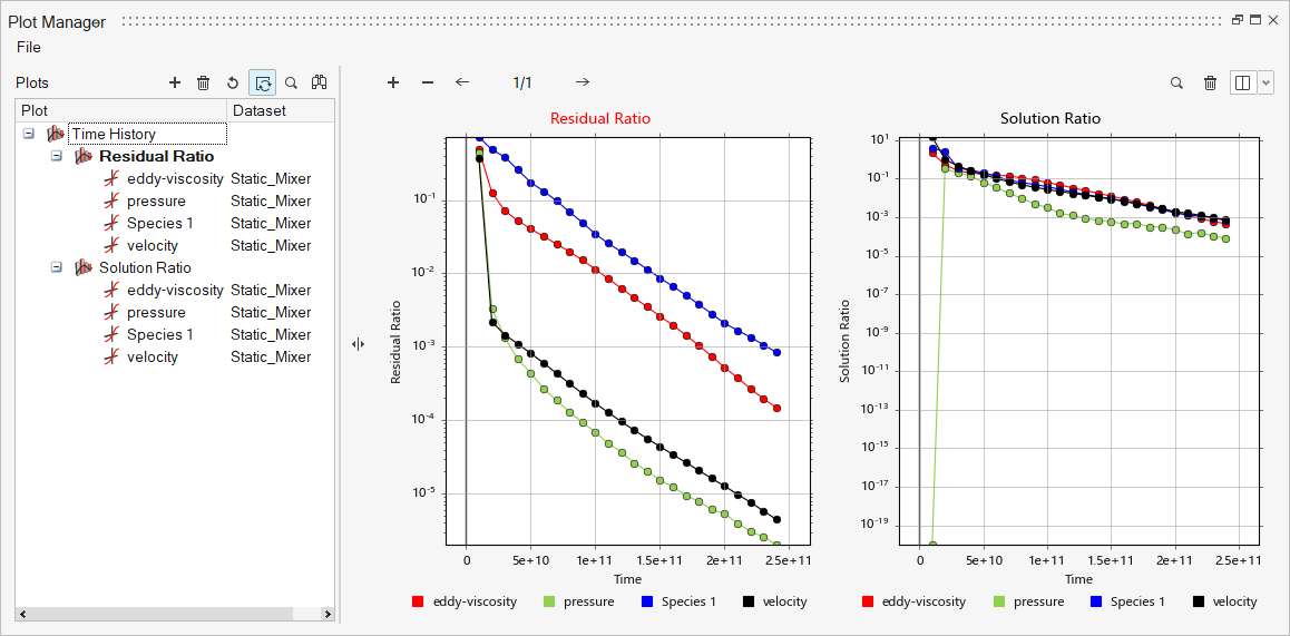
Post-Process with HyperMesh CFD Post
- Navigate to the Post ribbon.
-
From the Home tools, Files tool group, click the Open Model tool.
Figure 29.
- Open the AcuSolve .log file in your problem directory to load the results for post-processing.
-
Verify that the default step is set to Last in the
Reader Options dialog and then click
Import.
Figure 30. 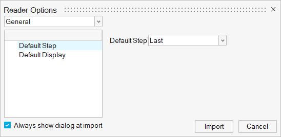
The solid and all the surfaces are loaded in the Post Browser.Figure 31. 
-
In the Post Browser, right-click Pipe
Wall and select Edit. Set the
transparency to around 80%.
Figure 32. 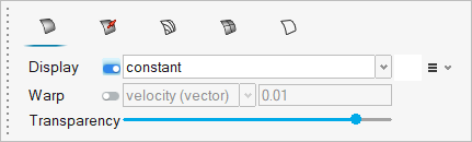
-
Similarly, edit the transparency of Fin Walls to around 30% .
Figure 33. 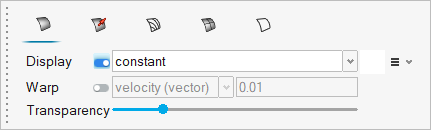
- Hide Outlet and Inlet S2.
-
Click the Slice Planes tool.
Figure 34. 
-
Select the x-z plane in the modeling window and then
click Calculate.
Figure 35. 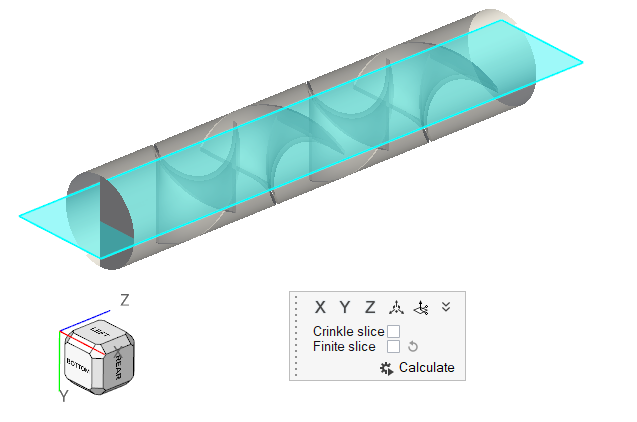
- In the display properties microdialog, set the display to species 1 and activate the Legend toggle.
-
Click
 to reset the legend.
-
Click
 and set the Colormap name to Rainbow
Uniform.
and set the Colormap name to Rainbow
Uniform.
Figure 36. 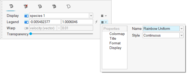
-
Click on the guide bar.
The plot below shows the mixing effectiveness as the maximum value of species 1 is reduced to 0.7 at the outlet, while the minimum value of species 1 is increased to 0.3.
Figure 37. 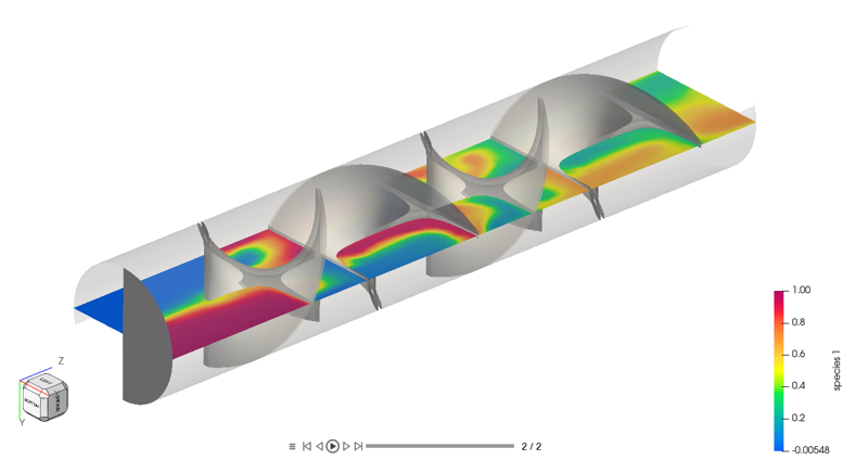
Prepare Particle Trace Attributes for AcuTrace
Define Particle Trace Parameters for Static Analysis
- Navigate to the AcuTrace ribbon.
-
Click the Setup tool.
Figure 38. 
- Click Problem definition and set the Particle type to Finite Mass.
- For the AcuSolve working directory, select the ACUSIM.DIR (flow results) folder in your problem directory.
- Make sure the Flow field type set to Static.
-
Disable Mesh motion if it not disabled already.
Figure 39. 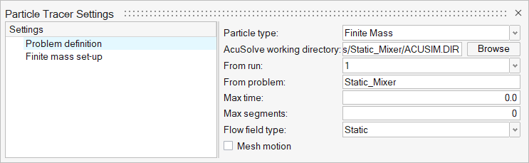
-
Click Finite mass set-up and leave all the parameters as
shown below.
Figure 40. 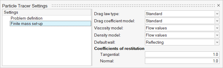
- Close the dialog.
Define Particle Seeds
-
Click the Seeds tool.
Figure 41. 
-
In the Seed location window, click
 .
.
- Browse to the location where you saved seeds1.csv and seeds2.csv.
-
Select seeds1.csv file and click
Open.
This accounts for the particles being fed from Inlet S1.
Figure 42. 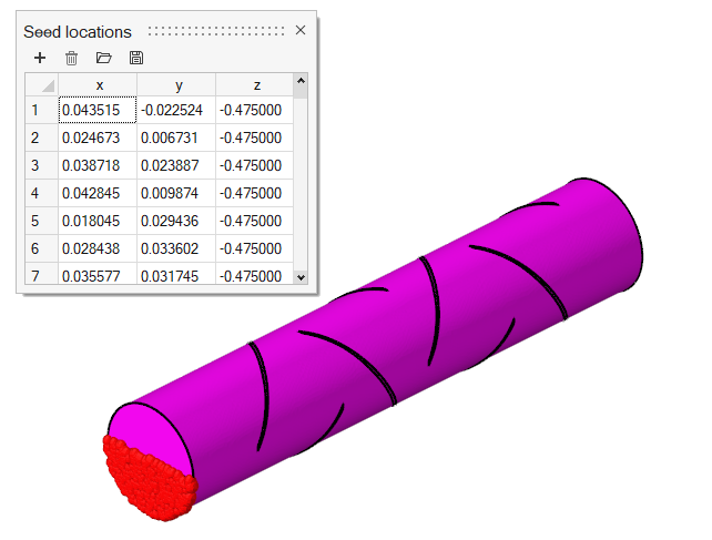
-
Click Parameters on the guide bar
and enter the following details.
Figure 43. 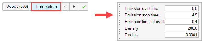
-
Click on the guide bar to execute
the changes.
- Right-click Particle Seeds in the legend and select Rename. Change the name to Inlet S1 Seeds.
-
Repeat the same process and open seeds2.csv.
Figure 44. 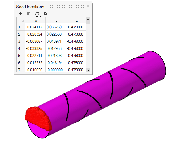
-
Click Parameters on the guide bar
and enter the following details.
Figure 45. 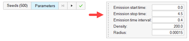
-
Click on the guide bar to execute
the changes.
- Right-click Particle Seeds in the legend and select Rename. Change the name to Inlet S2 Seeds.
-
On the guide bar, click
to execute
the command and exit the tool.
Define Finite Mass Boundary Conditions
-
Click the Reflecting tool.
Figure 46. 
-
In the Boundary Conditions window, select the
Pipe Wall and then set the Coefficients of
restitution values to 0.2.
Figure 47. 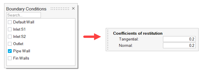
-
Click on the guide bar to execute
the changes.
- Right-click Reflecting Wall in the legend and select Rename. Change the name to Pipe Wall.
-
In the Boundary Conditions window, select the
Fin Walls and then set the Coefficients of
restitution values to 0.8.
Figure 48. 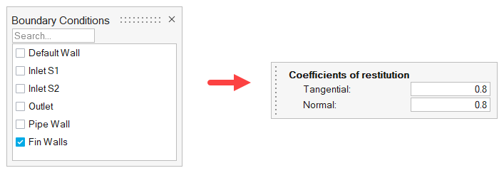
-
Click on the guide bar to execute
the changes.
- Right-click Reflecting Wall in the legend and select Rename. Change the name to Fin Walls.
-
On the guide bar, click
to execute
the command and exit the tool.
-
Click the Stopping tool.
Figure 49. 
- In the Boundary Conditions window, select the Outlet.
-
Click on the guide bar then .
Define Output Parameters
-
Click the Output tool.
Figure 50. 
-
Check Trace output and enter the values shown
below.
Figure 51. 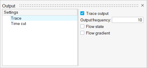
-
Click the Time cut setting and enter the values shown
below.
Figure 52. 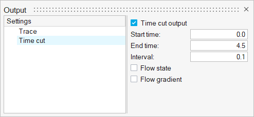
- Close the dialog.
Run AcuTrace
-
Click the Run tool.
Figure 53. 
- Check that acuRunTrace.bat is pointing to the correct path: <installation_directory>\hwcfdsolvers\acusolve\win64\bin\acuRunTrace.bat.
- Set the Parallel processing option to Intel MPI.
- Optional: Set the number of processors to 4 or 8 based on availability.
-
Leave the remaining options as default and click Run to
launch AcuTrace.
Figure 54. 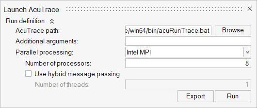
Convert Results for Ensight
-
Click the Convert tool.
Figure 55. 
The AcuTrace Data Translator window opens. - Browse to the location where the AcuTrace .log file (*.tlog) is located.
- Set the Output format to Ensight.
-
Set Data type to Time Cut.
Figure 56. 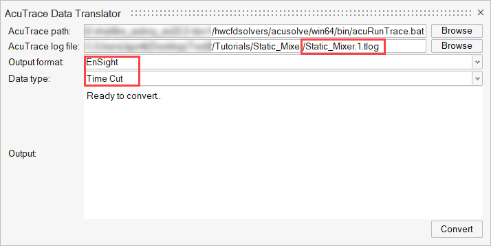
-
Click Convert.
Once the conversion is successful, it generates two Ensight result files.
Figure 57. 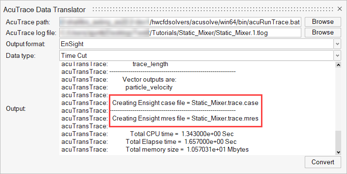
- Close the dialog.
Post-Process the Ensight File
- Navigate to the Post ribbon.
-
From the Home tools, Files tool group, click the Open Model tool.
Figure 58.
-
Open the Ensight case file (static_mixer.trace.case) in
your problem directory to load the results for post-processing.
Note: A warning opens wherein if some results were previously loaded it will try to remove the results first then load the current results. Click Continue.The solid and all the surfaces along with the Particles are loaded in the Post Browser.
Figure 59. 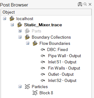
- In the Post Browser, turn off the display for all surfaces except for Pipe Wall and Fin Walls.
- Set the transparency for Fin Walls to around 30% and the transparency for Pipe Wall to around 80%.
- Right-click Block8 under Particles and select Edit.
-
Set the display to Radius. Click and set the point radius to
0.003.
Figure 60. 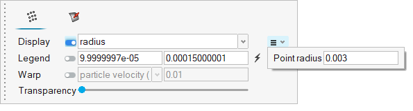
-
Activate the Legend toggle and click to refresh the range.
-
Click and set the colormap name to Rainbow
Desaturated, the colormap style to
Filled, and the number of colors to
2.
Figure 61. 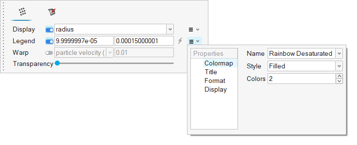
-
Switch to the Display properties. Set the Orientation to
Horizontal and select the Lower
Center button.
Figure 62. 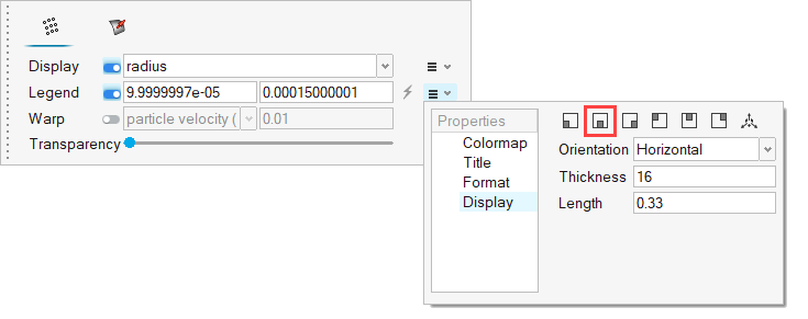
-
Click the Isometric face on the View Cube to align the
model.
Figure 63. 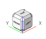
-
Rotate the model as shown in below figure such that you can view the particles
movement inside the domain more precisely.
Figure 64. 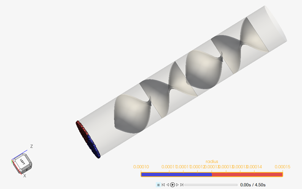
-
Click
 at the bottom of the modeling window to view a live animation of the flow.
Figure 65. 
-
Save the animation.
- Go to .
-
Click
 and uncheck Include mouse
cursor.
and uncheck Include mouse
cursor.
- Set the frame rate to 30.
-
Click
 on the toolbar then drag over the area you
want to record.
on the toolbar then drag over the area you
want to record.
-
Click
 to begin recording and the same icon to
stop recording.
to begin recording and the same icon to
stop recording.
- Name the file and save it.