
ACU-T: 2000 Turbulent Flow in a Mixing Elbow
Tutorial Level: Beginner
Prerequisites
Prior to starting this tutorial, you should have already run through the introductory tutorial, ACU-T: 1000 UI Introduction. To run this simulation, you will need access to a licensed version of HyperMesh CFD and AcuSolve.
Problem Description
The problem characteristics shown here determine if the flow is laminar or turbulent by calculating the Reynolds number in the pipe. The diameter of the large inlet is 0.1 m, and the inlet velocity (v) is 0.4 m/s. The diameter of the small inlet is 0.025 m, and the inlet velocity is 1.2 m/s.

The fluid in this problem is water with the following properties that do not change with temperature: a density (ρ) of 1000 kg/m3 and a molecular viscosity (μ) of 1 X 10⁻³ kg/m-sec.
Based on mass conservation, the combined flow rate (Q) yields a pipe velocity of 0.475 m/s downstream of the small inlet. The following equations are used to calculate the pipe velocity:
This value is useful in determining the Reynolds number, which in turn can be used to determine if the flow should be modeled as turbulent, or if it should be modeled as laminar.
In order to determine whether the modeled flow would be turbulent or whether it would be laminar, the Reynolds number (Re) should be calculated. The Reynolds number is given by:
where ρ is the fluid density, V is the fluid velocity, D is the diameter of the flow region, and μ is the molecular viscosity of the fluid. When the Reynolds number is above 4,000, it is generally accepted that flow should be modeled as turbulent.
The Reynolds numbers of 40,000 at the large inlet, 30,000 at the small inlet, and 47,500 for the combined flow indicate that the flow is turbulent throughout the flow domain. The simulation will be set up to model steady state, turbulent flow.
Start HyperMesh CFD and Open the HyperMesh Database
- Start HyperMesh CFD from the Windows Start menu by clicking .
-
From the Home tools, Files tool group, click the Open Model tool.
Figure 2. 
The Open File dialog opens. - Browse to the directory where you saved the model file. Select the HyperMesh file ACU-T2000_MixingElbow.hm and click Open.
- Click .
-
Create a new directory named MixingElbow_Turbulent and navigate into this directory.
This will be the working directory and all the files related to the simulation will be stored in this location.
- Enter MixingElbow as the file name for the database, or choose any name of your preference.
- Click Save to create the database.
Validate the Geometry
-
From the Geometry ribbon, click the Validate tool.
Figure 3. 
The Validate tool scans through the entire model, performs checks on the surfaces and solids, and flags any defects in the geometry, such as free edges, closed shells, intersections, duplicates, and slivers.The current model does not have any of the issues mentioned above. Alternatively, if any issues are found, they are indicated by the number in the brackets adjacent to the tool name.
Observe that a blue check mark appears on the top-left corner of the Validate icon. This indicates that the tool found no issues with the geometry model.Figure 4. 
- Press Esc or right-click in the modeling window and swipe the cursor over the green check mark from right to left.
- Save the database.
Set Up the Problem
Set Up the Simulation Parameters and Solver Settings
-
From the Flow ribbon, click the Physics tool.
Figure 5. 
The Setup dialog opens. -
Under the Physics models setting:
Figure 6. 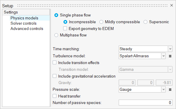
-
Click the Solver controls setting and verify that the
parameters are set as shown in the figure below.
Figure 7. 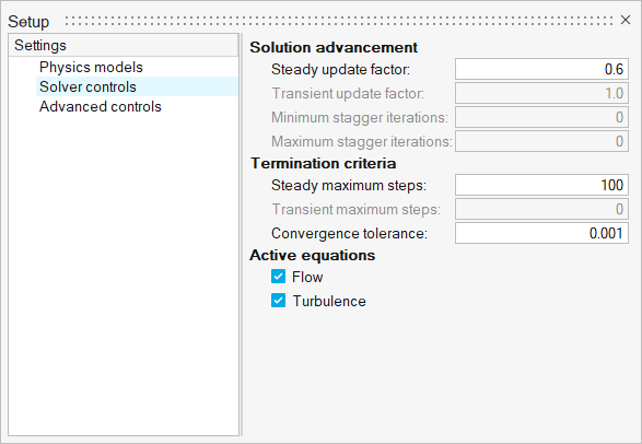
- Close the dialog and save the model.
Assign Material Properties
-
From the Flow ribbon, click the Material tool.
Figure 8. 
-
Select the model body.
The entire solid is highlighted.
Figure 9. 
- In the microdialog, click the drop-down menu next to Material and select Water.
-
On the guide bar, click
 to execute
the command and exit the tool.
to execute
the command and exit the tool.
Assign Flow Boundary Conditions
Set Boundary Conditions for the Large Inlet
-
From the Flow ribbon, Profiled
tool group, click the Profiled Inlet tool.
Figure 10. 
-
Click the face of the large inlet.
Figure 11. 
-
In the microdialog, enter a value of
0.4 m/s for Average velocity.
Figure 12. 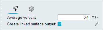
-
Rename the inlet.
- From the legend on the left side of the modeling window, double-click Inlet.
- Type Large_Inlet and press Enter.
-
On the guide bar, click
 to execute the command and remain in the
tool.
Note: The number of inlets created appears in parenthesis on the top-right of the Profiled tool icon.
to execute the command and remain in the
tool.
Note: The number of inlets created appears in parenthesis on the top-right of the Profiled tool icon.
Set Boundary Conditions for the Small Inlet
-
Click the face of the small inlet.
Figure 13. 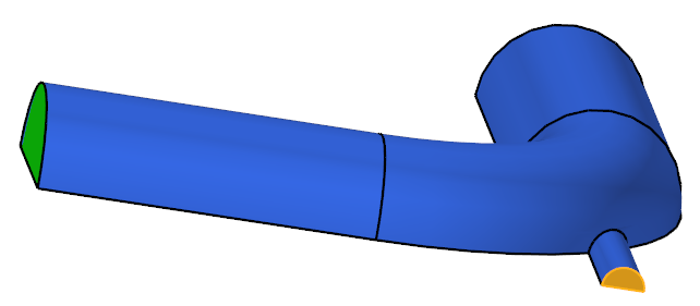
-
In the microdialog, enter a value of
1.2 m/s for Average velocity.
Figure 14. 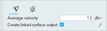
-
Rename the inlet.
- From the legend on the left side of the modeling window, double-click Inlet.
- Type Small_Inlet and press Enter.
-
On the guide bar, click
to execute
the command and exit the tool.
Set Boundary Conditions for the Outlet
-
From the Flow ribbon, click the Outlet tool.
Figure 15. 
-
Click the face of the outlet.
Figure 16. 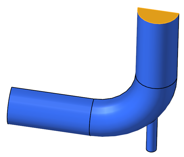
-
In the microdialog, make sure the
Static pressure is 0 Pa and the Pressure loss factor is also 0.
Figure 17. 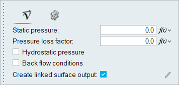
-
On the guide bar, click
to execute
the command and exit the tool.
Set Boundary Conditions for the Symmetry Plane
This geometry is symmetric about the XY midplane, and can therefore be modeled with half of the geometry. In order to take advantage of this, the midplane needs to be identified as a symmetry plane. The symmetry boundary condition enforces constraints such that the flow field from one side of the plane is a mirror image of that on the other side.
-
From the Flow ribbon, click the Symmetry tool.
Figure 18. 
-
Select the face of the symmetry plane.
Figure 19. 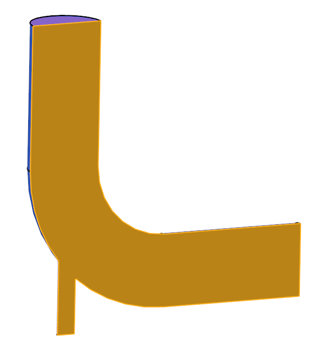
-
In the microdialog, accept the
default symmetry conditions.
Figure 20. 
-
On the guide bar, click
to execute
the command and exit the tool.
- Save the database.
Generate the Mesh
-
From the Mesh ribbon, click the
Volume tool.
Figure 21. 
The Meshing Operations dialog opens.Note: If the model has not been validated, you are prompted to create the simulation model before running the batch mesh. - Check that the Average element size is 0.025 m.
-
Accept all other default parameters.
Figure 22. 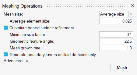
-
Click Mesh.
The Run Status dialog opens. Once the run is complete, the status is updated and you can close the dialog.Tip: Right-click the mesh job and select View log file to view a summary of the meshing process.
-
From the back side of the model, observe the refined mesh around the small
inlet.
Figure 23. 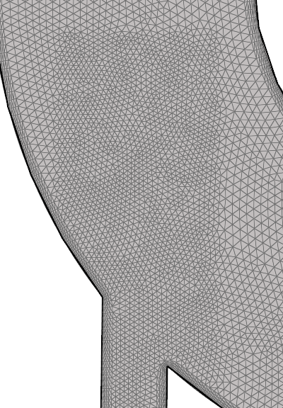
Run AcuSolve
-
From the Solution ribbon, click the Run tool.
Figure 24. 
The Launch AcuSolve dialog opens. - Set the Parallel processing option to Intel MPI.
- Optional: Set the number of processors to 4 or 8 based on availability.
- Deactivate the Automatically define pressure reference option.
-
Leave the remaining options as default and click
Run to launch AcuSolve.
Figure 25. 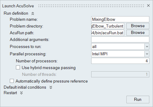
The Run Status dialog opens. Once the run is complete, the status is updated and you can close the dialog.Tip: While AcuSolve is running, right-click the AcuSolve job in the Run Status dialog and select View Log File to monitor the solution process.
Post-Process the Results with HM-CFD Post
- Once the solution is completed, navigate to the Post ribbon.
- From the menu bar, click .
-
Select the AcuSolve
.log file in your problem
directory to load the results for post-processing.
The solid and all the surfaces are loaded in the Post Browser.
- Isolate the Symmetry flow boundary in the Post Browser.
- Right-click Symmetry and select Edit.
- In the display properties microdialog, set the display to velocity and activate the Legend toggle.
-
Click
 and set the Colormap Name to Rainbow
Uniform.
and set the Colormap Name to Rainbow
Uniform.
Figure 26. 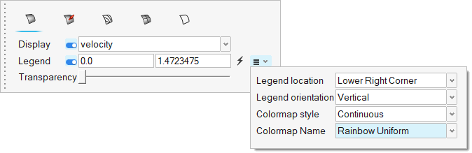
-
Click
 on the guide bar to show the velocity magnitude (m/s)
contour.
on the guide bar to show the velocity magnitude (m/s)
contour.
Figure 27. 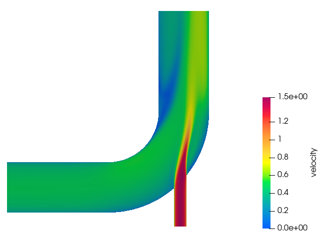
- Again, right-click the Symmetry and select Edit.
- Display the pressure (Pa).
-
Click
 to reset the range.
Figure 28. 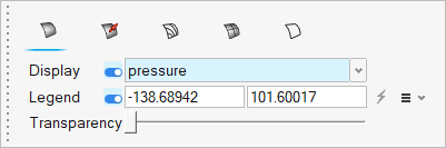
-
Click on the guide bar to show the pressure (Pa)
contours.
Figure 29. 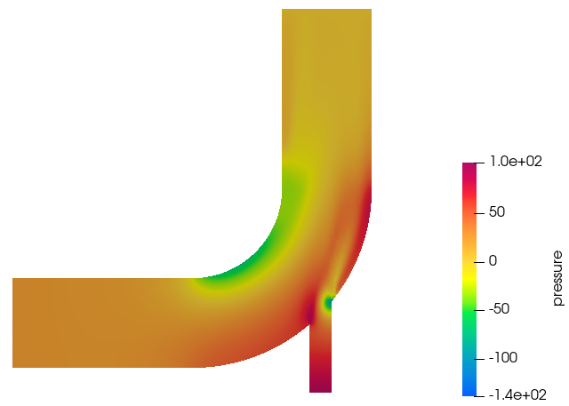
Summary
In this tutorial, you worked through a basic workflow to set up a CFD model, carry out a CFD simulation, and post-process the results. You started by importing the model in HyperMesh CFD. Then, you defined the simulation parameters and launched AcuSolve directly from within HyperMesh CFD. Upon completion of the solution by AcuSolve, you used the Post ribbon to create contour plots.