Finite Volume Method (FVM)

This section describes the formulation and methodology of finite volume method to solve the governing equations on a computational domain. It also describes the cell centered and face centered approaches used for finite volume formulation.

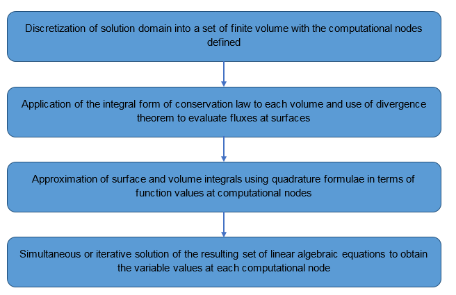
The finite volume formulation is based on the approximate solution of the integral form of the conservation equations. The problem domain is divided into a set of non overlapping control volumes referred to as finite volumes, where the variable of interest is usually taken at the centroid of the finite volume. The finite volume is also referred to as a cell or element.

The governing equations are integrated over each finite volume and interpolation profiles are assumed in order to describe the variation of the concerned variable of interest between the cell centroids. The resulting discretization equation expresses the conservation principle for the variable inside the finite volume.

The governing differential equations discussed in this manual each have a dependent variable that obeys a generalized conservation principle. If the dependent variable (scalar or vector) is denoted by

φ

, the generic differential equation is: (1)

\underset{T r a n s i e n t t e r m}{\underset{}{\frac{\partial (ρ φ)}{\partial t}}} + \underset{C o n v e c t i o n t e r m}{\underset{}{\nabla \cdot (ρ \vec{u} φ)}} = \underset{D i f f u s i o n t e r m}{\underset{}{\nabla \cdot (ϵ \nabla φ)}} + \underset{S o u r c e t e r m}{\underset{}{S_{φ}}}

where

$ϵ$ is the diffusion coefficient.
The transient term $\frac{\partial ρ φ}{\partial t}$ accounts for the rate of change of $φ$ inside the control volume.
The convection term $\nabla \cdot (ρ \vec{u} φ)$ accounts for the transport of $φ$ due to the velocity field $\vec{u}$ .
The diffusion term $\nabla \cdot (ϵ \nabla φ)$ accounts for the transport of $φ$ due to its gradients.
The source term $S_{φ}$ accounts for any sources or sinks that affect the quantity $φ$ .

When the above equation is integrated over a three dimensional control volume it yields (2)

\int_{C V}^{} \frac{\partial (ρ φ)}{\partial t} d V + \int_{C V}^{} \nabla \cdot (ρ \vec{u} φ) d V = \int_{C V}^{} \nabla \cdot (ϵ \nabla φ) d V + \int_{C V}^{} S_{φ} d V

The divergence terms (convection and diffusion) can be converted into surface integrals using Gauss divergence theorem and the above equation can be rewritten as (3)

\frac{\partial}{\partial t} \int_{C V}^{} ρ φ d V + \oint_{S}^{} \hat{n} \cdot (ρ \vec{u} φ) d S = \oint_{S}^{} \hat{n} \cdot (ϵ \nabla φ) d S + \int_{C V}^{} S_{φ} d V

where

$\hat{n}$ is the unit vector normal to the surface $d A$
$S$ is the boundary of the control volume
$\hat{n} \cdot (ρ \vec{u} φ)$ is the convective flux of $φ$ across the boundary $d S$
$\hat{n} \cdot (ϵ \nabla φ)$ is the diffusive flux of $φ$ across the boundary $d S$

The integral conservation in the scalar transport equation applies to each control volume as well as the complete solution domain thus satisfying the global conservation of quantities such as mass, momentum and energy. These quantities can be evaluated as fluxes at the surfaces of each control volume.

In order to obtain an algebraic (discretised) equation for each control volume the surface and volume integrals are approximated using quadrature formulae in terms of function values at the storage location. This may require values of variable at points other than the computational nodes of the control volume. Values at these locations are obtained using interpolation schemes.

The overall finite volume approach involves the following steps.

There are two common approaches to finite volume discretization.

Cell centered approach: The domain is defined by a suitable grid of finite volumes and the computational nodes are assigned at the centroid of the control volumes.
Face/Node centered approach: The domain is first defined by a set of nodes and control volumes are constructed around these nodes as cell centers such that the faces of the control volume lie between these nodes.

The cell centered approach and node centered approach have nearly the same accuracy and efficiency for most of the cases which use a structured grid.

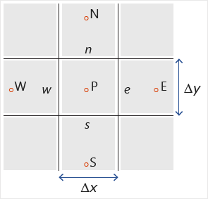
To illustrate how the conservation equations in CFD can be discretised using finite volume method an example involving the steady transport of x-momentum in a uniform 2D rectangular grid can be considered:

A cell centered approach is employed with the points P, W, E, N, S representing the cell centers and the notations n, e, s, w representing the faces of cell P. The notation N (n), E(e), S(s), W(w) represent the north, east, south and west directions, respectively.

The velocity

u

is stored at the nodes N, E, S, W and it is represented as

u_{N}

u_{E}

u_{S}

u_{W}

, respectively. The finite volume approximation starts by integrating the x-momentum equation over the control volume P. (4)

\iint_{V}^{} [\frac{\partial}{\partial x} (ρ u^{2}) + \frac{\partial}{\partial y} (ρ u v)] d x d y = - \iint_{V}^{} \frac{\partial p}{\partial x} d x d y

(5)

+ \iint_{V}^{} [\frac{\partial}{\partial x} (μ \frac{\partial u}{\partial x}) + \frac{\partial}{\partial y} (μ \frac{\partial u}{\partial y})] d x d y

This leads to: (6)

{[\int ρ u^{2} d y]}_{w}^{e} + {[\int ρ u v d x]}_{s}^{n} = {[\int μ \frac{\partial u}{\partial x} d y]}_{w}^{e} + {[\int μ \frac{\partial u}{\partial y} d x]}_{s}^{n} - \iint_{V}^{} \frac{\partial p}{\partial x} d x d y

Evaluation of Source Terms: The source terms can be approximated by evaluating them at cell centers and multiplying them by the volume of the cell.; $\iint_{V}^{} \frac{\partial p}{\partial x} d x d y \approx {(\frac{\partial p}{\partial x})}_{P} Δ x Δ y$; In the example considered the pressure gradient at center of cell P can be evaluated by interpolating the pressure values from surrounding nodes. Other source terms can be evaluated similarly, interpolating where necessary to estimate the cell center values.
Evaluation of Diffusive Fluxes: The diffusive fluxes can be approximated as; ${[\int μ \frac{\partial u}{\partial x} d y]}_{w}^{e} + {[\int μ \frac{\partial u}{\partial y} d x]}_{s}^{n} \approx {[μ \frac{\partial u}{\partial x} Δ y]}_{w}^{e} + {[μ \frac{\partial u}{\partial y} Δ x]}_{s}^{n}$; The gradients of velocity at the cell faces (e, w, n, s) can be approximated using central difference comprising of the cell center values. This results in diffusive fluxes being represented as; ${[\int μ \frac{\partial u}{\partial x} d y]}_{w}^{e} + {[\int μ \frac{\partial u}{\partial y} d x]}_{s}^{n} \approx {(μ Δ y)}_{e} \frac{u_{E} - u_{P}}{Δ x} - {(μ Δ y)}_{w} \frac{u_{P} - u_{W}}{Δ x}$; $- {(μ Δ y)}_{n} \frac{u_{N} - u_{P}}{Δ y} - {(μ Δ y)}_{s} \frac{u_{P} - u_{S}}{Δ y}$; The discretised equation which is second-order accurate takes the form; $a_{e} u_{E} + a_{w} u_{W} + a_{n} u_{N} + a_{s} u_{S} - a_{p} u_{P}$
Evaluation of Convective Fluxes: The convective fluxes can be approximated as; ${[\int ρ u^{2} d y]}_{w}^{e} + {[\int ρ u v d x]}_{s}^{n} \approx {[ρ u^{2} Δ y]}_{w}^{e} + {[ρ u v Δ x]}_{s}^{n}$; The discretised equation takes the form; $c_{e} u_{e} - c_{w} u_{w} + c_{n} u_{n} - c_{s} u_{s}$; where $c_{e}$ , $c_{w}$ and so on are mass fluxes through the east, west, north and south faces.; The values of $u$ at cell faces need to be obtained using appropriate interpolation schemes between the cell center values. A few examples of such schemes are linear interpolation (CDS), quadratic upwind interpolation (QUICK), total variation diminishing (TVD).