
Finite Difference Method (FDM)
This section describes the formulation and methodology of finite difference method to solve the governing equations on a computational domain.
The finite difference method is the oldest method for the numerical solution of partial differential equations. It is also the easiest to formulate and program for problems which have a simple geometry.
When calculating derivatives finite difference replaces the infinitesimal limiting process with a finite quantity. The derivative of a function at point expressed as:
is replaced by:
The preceding expression is commonly referred to as the forward difference approximation. This derivative can have more refined approximations using a number of approaches such as truncated Taylor series expansions and polynomial fitting.
The term gives an indication of the magnitude of the error as a function of the mesh spacing and is therefore termed as the order of magnitude of the finite difference method. In the above formulation, the finite difference approximation employed is first-order accurate. A second-order approximation would have the order of magnitude expressed as . Most of the finite difference methods used in practice are second-order accurate. An example of a second-order method is the central difference approximation of the first derivative. It is expressed as:
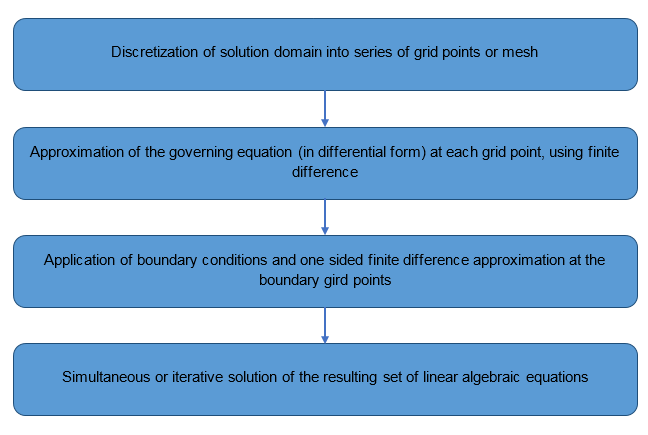
The finite difference formulation generally employs a structured grid. The most commonly used indices are , and for the grid lines at , and , respectively. The function value at such a grid point is expressed as .
Consider the one dimension advection-diffusion equation for a scalar quantity governed by
where is the specified velocity, is the density of the fluid and is the diffusivity.
If the domain is defined by the boundary and and the boundary conditions by and , the domain can be discretised (non-uniformly) by a total of grid points for the finite difference solution of the problem.
The diffusion term can be approximated using the central difference (both the inner and outer derivative) as:
The convection term can also be approximated using the central difference as:
If the grid is uniform and the values of density, velocity and coefficient of diffusion are constant throughout the domain the above equations reduce to:
The resulting set of linear algebraic equations can be solved to get the values of at the grid points.
Finite difference methods are advantageous for the numerical solution of partial differential equations because of their simplicity, efficiency and low computational cost. Their major drawback is their geometrical inflexibility, such as application on an unstructured grid or moving boundaries. Their formulation increases in complexity as the complexity of the domain increases.
The restrictions resulting from the above mentioned geometrical complexities can be alleviated by the use of methods such as grid transformation and immersed boundary techniques.