Induction machines - Efficiency maps vectorial UI
Positioning and objective
The aim of the test “Performance mapping – Sine wave – Motor – Efficiency map” is to characterize the behavior of the machine in the "Torque-Speed" area.
Input parameters like the “Maximum line current”, “Maximum Line-Line voltage”, and the desired “Maximum speed” of the machine are considered.
Only the Maximum Torque Per Volt command mode (MTPV) is available in this version. The Maximum Torque Per Amps command mode (MTPA) will be available as soon as possible.
Input parameters define the torque-speed area in which the evaluation of the machine’s behavior is performed.
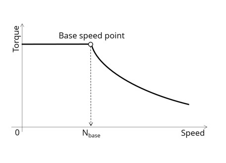 |
| Characterization of the corner point on the torque-speed curve |
Here is an overview of the test, given below.
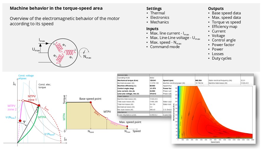 |
| Performance mapping / Efficiency map – Induction machine with squirrel cage - Inner rotor (IMSQ - IR) - Overview |
Main inputs, settings and outputs
- Inputs
The main user input parameters needed to perform this test are the maximum allowed supply line current, line-line voltage, the targeted maximum speed, and the command mode. Winding and cage temperatures must also be set.
When required, the location of the working points (single point or duty cycle) to be evaluated must be defined as inputs.
Warning:The default values of advanced inputs have been set to get the best compromise between accuracy and computation time.
Four advanced user input parameters allow adjusting the compromise between accuracy and computation time: the number of iterations for Kr evaluation, the number of computations for Jd-Jq, for speed, and for torque.
Note: It is possible to import the current inputs and results from the test “Characterization – Model – Motor – Maps”. This will save computation time related to the identification of the non-linear model; in other words, it will save the computation time related to the finite element solving, which generally represents the main part of the computation time of the test. - Settings
- Temperature of active components: winding and squirrel cage
- Definition of the power electronics parameters
- Definition of mechanical loss model parameters
- Import functionality
- Outputs
Tables, curves and maps are computed and displayed as illustrated below.
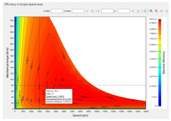
In the results, the performance of the machine at the base point (the base speed point) and for the maximum speed set by the user are presented. A set of curves (like Torque-Speed curve) and maps (like Efficiency map) are computed and displayed.
Here are below illustrations of some results that can be provided in the test.
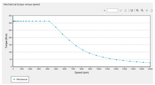 |
| Mechanical torque versus speed - Example |
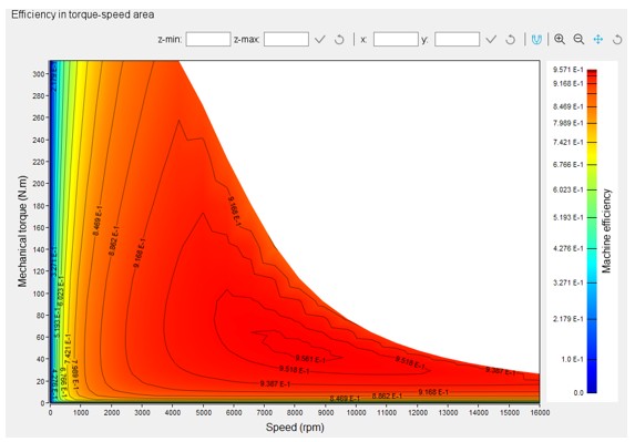 |
| Efficiency in torque-speed area - Example |
The second feature allows the user to define a duty cycle by giving a list of working points (speed, torque) versus time. The displayed results illustrate the machine performance over the considered duty cycle (mean, min, and max values).
The time variation of the main quantities is also displayed (mechanical torque, speed, control angle, current, voltage, power, efficiency, and losses).
All the corresponding points are displayed on the different maps provided. Each working point can be selected to visualize the corresponding main information.
 |
| A “Duty cycle” displayed on the efficiency map - Example |
- Machine performance at the base speed point, at the maximum speed and at a user working point
- Duty cycle
- Torque-speed curves
- Mechanical torque versus speed
- Current versus speed (J, Jd, Jq)
- Voltage versus speed (V, Vd, Vq)
- Control angle versus speed
- Power versus speed (Mechanical power, Machine electrical power, System electrical power)
- Power factor versus speed
- Losses versus speed (Total machine and system, Stator Joule, Rotor Joule, Stator iron, Mechanical, Power electronics)
- Rotor Joule losses versus speed (Rotor Joule, Bars Joule, End ring C.S. Joule, End ring O.C.S. Joule)
- Slip versus speed
- Frequency versus speed (Slip frequency, Stator frequency)
- Inductances versus speed (Ld static, Lq static)
- Saliency versus speed
- Characteristic curves
- Electromagnetic torque versus current and control angle () according to base speed point
- Characteristic curves in Jd-Jq area - Evolution of the working points in Jd-Jq plane, with iso-torque, iso-current and iso-voltage.
Brief introduction about the main principles of computation
- Raw data provided by the solving of the test “Characterization - Model - Motor - Maps”
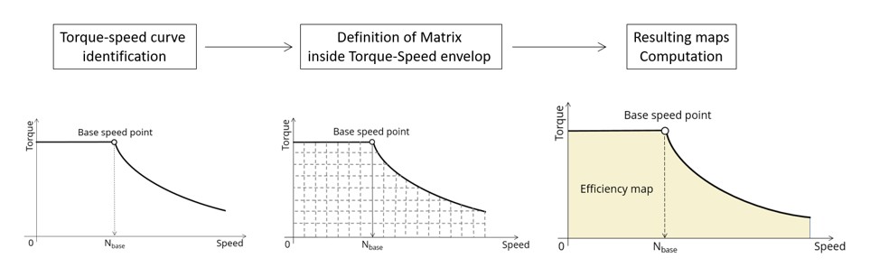
- Principle for computing the torque-speed curves and maps
- MTPV vector command
- Raw data and Park’s model
The first step corresponds to the solving of the test “Characterization - Model - Motor - Maps” which consists of computing the raw data that characterize the machine in the Jd-Jq plane. This is done using Finite Element modelling (Flux® – Magnetostatic application).
For additional information, please refer to the explanation above.
- Identification process for the torque-speed curves and maps under
vector control
Below are the three main steps involved in building the efficiency map and other associated results.
These steps are based on the computed raw data (see previous section) with optimization processes.
- Building of the torque-speed curve and other associated results
- Define the grid in the area under the torque-speed curve
- Building of the efficiency map and other associated results
Main steps of the computation algorithm - MTPV vector command
The Maximum Torque Per Voltage command mode (MTPV) allows to compute the torque-speed curve, which corresponds to the maximum potential of mechanical torque (or mechanical power) of a motor from the base speed point to the maximum speed point.
This command mode shows the full potential of the machine, but it is also the most difficult command mode to implement in terms of control and drive.
This command is used to compute the torque speed curve from the base speed point to the maximum speed.
Upstream the base speed point, the torque speed curve is obtained by imposing the useful torque computed at the base speed point and by maximizing the efficiency.
The maps bounded by the considered torque-speed curve are computed by maximizing the efficiency for each paired value (Torque, Speed).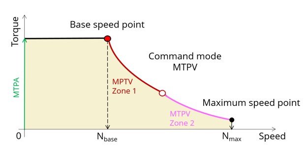
Torque speed curve with MTPV command mode Over the speed range [Nbase, Nmax.] we distinguish two main zones, the Zone 1 commonly called “Flux weakening” and the Zone 2 commonly called “MTPV curve”.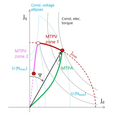
Evaluation of the working point in Jd-Jq plane by considering iso-torque, iso-current and iso-voltage In the first zone (MTPV zone 1), the maximization of the mechanical torque for a given speed is reached by keeping the maximum values of voltage and current, and by driving the control angle (Ψ). In a second zone (MTPV zone 2), the maximization of the mechanical torque is reached by keeping the maximum values of voltage and by decreasing the line current below the maximum allowed value and by driving the control angle (Ψ). In FluxMotor, the MTPV label is used to mention the combination of these two zones (for both, the maximum torque is computed, at the maximum voltage available). The optimization process automatically deduces the best working zone according to the following constraints: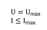
With MTPV command mode the mechanical power is not imposed over the speed range [Nb, Nmax.] as commonly done.
In fact, over Zone 1 and Zone 2, the MTPV command mode imposes to maximize the mechanical torque at maximum voltage. Maximizing the mechanical torque at an imposed speed is equivalent to maximizing the mechanical power.
In conclusion, the MTPV command mode allows to spotlight the potential of mechanical power that the machine can provide over a speed range from the base speed point to the maximum speed point with a given maximum line-line voltage and a maximum line current.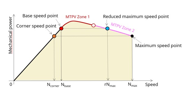
Mechanical power with MTPV command mode Thanks to the MTPV results, we can easily deduce the maximum mechanical power that the machine is able to provide over a range of speed.
For examples, referring to the previous figure:
- Raw data and Park’s model
- If we want to impose the mechanical power obtained at the maximum point speed, we can easily deduce the bound at low speed. We called this point the corner speed point (Orange point on the previous figure).
- If we want to impose the mechanical power obtained at the base speed point, we are able to deduce the bound at high speed. We called this point the reduced maximum speed point (Blue point on the previous figure).