Parabolic Equation Method
The parabolic equation method efficiently describes diffraction and forward-scattering processes in inhomogeneous terrains.
Due to the limited accuracy of the empirical models, there is a need for methods which describe diffraction and forward-scattering processes in inhomogeneous terrain, thus the effect of the terrain to the large-scale variation. Therefore, different full wave approaches have been investigated, and one efficient possibility is the parabolic equation method.
This method employs a numerical evaluation of the parabolic equation (PE) to compute the field strength in a macro-cellular area based on terrain data. Because the different propagation mechanisms (free space propagation, reflection and diffraction) are implicitly considered this model is very accurate. Due to the sophisticated algorithm, the computation time is quite long in comparison to the empirical models.
Basic Principles
Figure 1 shows the vertical terrain section and the computation domain of the PE model.
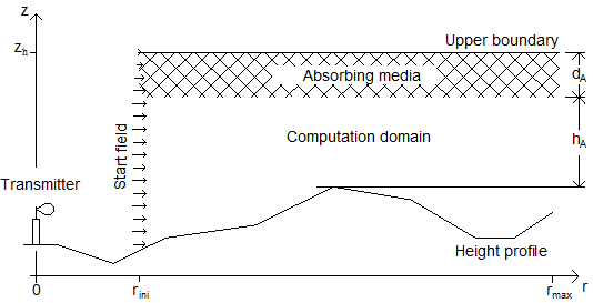
Neglecting backward propagation and assuming a rotationally symmetric problem, a partial differential equation of parabolic type out of the Maxwell equations can be derived:
This so-called standard parabolic equation (SPE) leads to valid results if the propagation angle with respect to the horizon is in the range, –15° to 15°. Therefore the PE must not be used in the vicinity of the transmitter.
A finite difference technique solves the PE in the computation domain using an iterative method. In WinProp the required start field at is computed using free space propagation and a single ground reflection ray.
Atmosphere
Among the parameters for Parabolic Equations you can choose whether to include atmospheric effects. The option Constant dielectricity performs a free-space simulation while the option Predefined height depending dielectricity assumes a standard atmosphere based on the following formula:
Absorbing Media
As the implementation of a transparent boundary condition at the top of the computation domain yielded too high computation times, an absorbing medium is used instead to avoid reflections at the upper boundary. Having a width of about wavelengths, the absorbing medium works well for all frequencies if an adequate distance to the highest terrain point is assumed.
The prediction plot in Figure 2 shows the field in the artificial absorbing medium above the dotted line.

Impedance Boundary at the Ground
For all parabolic equations calculations, the conductivity and dielectric permittivity of the ground surface is taken into account. Three variations how to model the impedance boundary condition are presented here.
- Discrete terrain approximation
A step-like height profile is assumed in Figure 3, which leads to the simplified Leontovich boundary condition.
Figure 3. Step-like height profile approximation. 
Due to numerical instabilities of this method, the radial step size of the computation grid is reduced at down-sloping ground automatically.
- Continuous terrain approximation
By setting appropriate values for the complex wave number , the ground is modeled as if it is a part of the atmosphere. Together with a variable step size this approach is very robust but does not match the boundary condition exactly because abrupt alterations of the atmospheric medium are not allowed when using the parabolic approximation.
- Terrain profile approximation with coordinate transformation
Another possibility to prevent numerical instabilities is the transformation of the irregular computation domain to a rectangular area as shown in Figure 4 for down-sloping ground.
Figure 4. Transformation of the computation domain. 
Therefore the coordinate transformation
Because of the distortion of the computation grid, the transformation should only be used for slight hilly terrains.
Wide Angle Parabolic Equation
The disadvantage of the small valid propagation angle of the standard parabolic equation can be remedied if an extended parabolic approximation of the Maxwell equations is used.
Therewith propagation angles up to about 40° are acceptable. The additional terms do hardly prolong the computation time and thus the wide angle PE should be preferred.