Determination of the Dominant Paths
The determination of dominant paths and the discarding of non-dominant paths can save time, but also compromise accuracy. Use specific settings to control the accuracy and prediction time.
In a first step, the sequence of the transmitted walls and rooms passed by the dominant path must be determined. Therefore an analysis of the database is mandatory. In the database, only information of the walls and the material of the walls is given, and no information about rooms is available. Therefore, rooms must be determined in a first step. After this initial step, a tree of the room-structure is computed as shown in Figure 1.
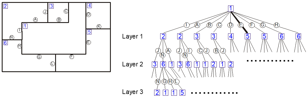
The root of the tree corresponds to the room in which the transmitter is placed. The first layer contains all neighboring rooms. If there are different walls between the transmitter room and the neighboring rooms (for example, wall E and F between room 1 and 5), the neighboring room is placed in this layer of the tree as many times as there are coupling walls between the rooms. After this first layer of the tree, the second layer is determined similarly, thus all neighboring rooms (and coupling walls) are branches of the corresponding rooms of the first layer. The tree contains as many layers as necessary for completeness, thus each room of the building must occur in the tree at least once.
After the determination of the tree, the dominant paths between the transmitter and the receiver can be computed very easily because if the receiver is located in room i, the tree must only be examined for room i. If room i is found in the tree, the corresponding dominant path can be determined by following all branches back to the root of the tree. For example, the path to room 5 through wall E is highlighted in Figure 1 to show the determination of the paths.
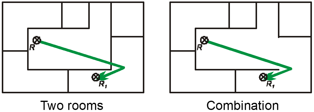
The coordinates of the path are always computed with the same algorithm, independent of the number of transmitted walls and passed rooms. This is only possible by combining all passed rooms to one room for the determination of the path. This is shown in Figure 2 for a given dominant path. Rooms 1 and 5 are combined, erasing wall E (names of the walls and rooms are given in Figure 1). Subsequently, the situation becomes similar to the situation where the receiver and the transmitter are located in the same room. The solution for the determination of the path inside a single room is described in the following section.
Path Determination in a Single Room
- Line of sight
- Obstructed line of sight
In the first case (line of sight) the determination of the dominant path is easy because it corresponds to the direct ray between the two points. The second case (obstructed line of sight) is a bit more complicated. In a first step, all the corners of the room get a number and are arranged into two lists, one containing all convex corners and the second list all concave corners (see Figure 3).
The concave corners are not used for determining the path, and thus the path between the two points must pass different convex corners (at least one convex corner). For the corners of the room, two trees are generated, as shown in Figure 3.
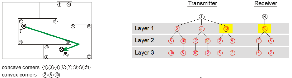
Two trees are necessary, one for the transmitter and one for the receiver. If there is a line of sight between the transmitter (receiver) and a convex corner, this corner is put in the first layer of the tree. The second layer consists of all convex corners which are visible (by a line of sight) from the corners in the first layer.
Subsequently, the determination of the path can be readily determined because it is only necessary to compare the trees for the transmitter and the receiver. If the same corner number is encountered on the first layer in both trees, the path leads via this corner (for example, corner 10 in Figure 3). If there are different numbers, the second layer in both trees must be compared to the first layer in the other tree, and if the same number is encountered here, then the path leads via this corner and the corresponding corner in the first layer. If no path is found at this level, the corners in the second layers of both trees are compared. This is done until the same number in both trees is encountered.
In the last step, the dominant path must be modified to be independent of the exact location of the corners, as mentioned above. Therefore the path is moved inside the room, depending on the angle of the corner and the distance to the next wall.
The option, Layers deeper than optimal path layer, determines how many layers deeper than the optimal layer of the room tree should be used for the path determination. A minimum and a maximum value can be specified. Appropriate values for min are 1 – 3 (default 2) and for max, 2 – 4 (default 3).
The option, Threshold for consideration of paths, defines the maximum difference (in dB) between the best path and the path under consideration: when this threshold is (not) exceeded the path under consideration is discarded (considered). Appropriate values are 2 – 6 dB, the default value is 3 dB.
If the box, Consider 3D path determination, is selected (default), then a rigorous 3D path search is performed. Otherwise only a 2D search is performed, leading to reduced accuracy.
If the box, Consider outdoor paths, is selected paths that exit the
building and re-enter
are also considered. Selecting the box could increase the
accuracy in some building structures where the propagation through the outdoor area is an
important part of the coverage, but it also increases the computation time.
Path Selection Criteria
The different path selection criteria parameters are described in Table 1:
| LP | Allows changing the weighting of the path loss (free space loss) that was computed for the rays. The default value is 1. A larger value increases the weight of the path loss. |
| LT | Allows changing the weighting of the transmission loss (due to the walls) that was computed for the rays. The default value is 1. A larger value increases the weight of the transmission loss. |
| LI | Allows changing the weighting of the interaction loss (due to diffraction) that was computed for the rays. The default value is 1,5. A larger value increases the weight of the interaction loss. |
| LW | Allows changing the weighting of the computed wave guiding gain (due to long parallel walls, for example, in corridors) that was computed for the rays. The default value is 2. A larger value increases the weight of the wave guiding gain. |
| nl | This is an additional correction factor (> 0) which allows considering an additional loss depending on the number of interactions. Appropriate values are between 0 and 2. |
| nmin | This is an additional correction factor (> 0) which allows considering an additional gain for the pixels that are reached in the first layer of the room tree. This is suggestive if these pixels are predicted with a too pessimistic value due to the building structure. Appropriate values are between 0 and 2. |
Share of the Empirical and Neural Model
In the current version, predictions with a neural part > 0 % are not possible. This empirical model allows an accurate prediction with moderate computation time. The dependency on the database accuracy is low, but a complex room detection is required, which determines all existing rooms and corridors. The computation time is moderate because only small parts of the prediction are preprocessed, and every propagation path is analytically determined. Still, it is much faster than the standard ray-tracing, as only the dominant paths are determined.