Directional Characteristic of Antennas
Commercial antennas do not radiate the same power density in all directions (in contrast to the isotropic radiator). There are always directions with higher power density and others with smaller power density.
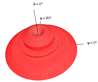
The direction with the highest power density is called the main direction. The antenna pattern describes the dependency of the radiation on the direction. It shows amplitude, phase and polarization assuming far field conditions (far away from the antenna itself). Spherical coordinates , and are used to describe the antenna pattern. As the distance is not relevant in the far field, the antenna pattern itself is a function of the angles and .
The pattern of real antennas depends additionally on the frequency. So, for different frequencies, different patterns must be used.
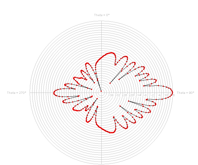
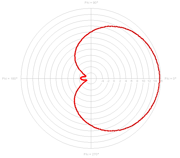
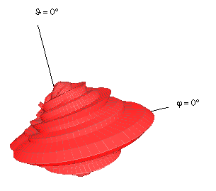
Often the radiation of the antenna is only measured in the horizontal and in the vertical plane. This reduces the effort and describes the antenna for most applications. Only accurate wave propagation models (like ray-optical models) will benefit from 3D antenna patterns.
| Vertical Pattern | Horizontal Pattern | 3D Representation |
|---|---|---|
|
|
|
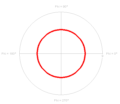
| Vertical Pattern | Horizontal Pattern | 3D Representation |
|---|---|---|
|
|
|
|
As the power density is proportional to the electric field strength , often the electric field strength is used to describe the antenna pattern. Usually, the pattern is normalized to its maximum value, for example:
Since, in the general case, elliptical polarization is present in the far field, both antenna patterns of the orthogonal polarization, and , are needed for the description of the directional characteristics of the antenna. and is generally normalized on the maximum value of the highest component: