The temperature on the inside surface of the pipe is 60 °C. The outside surface is
exposed to the surrounding air, which is at 20 °C. The temperature distribution
within the pipe can be determined by solving the linear steady state heat conduction
and convection solution.Figure 1. Model Review
The following exercises are included:
Create the thermal material and property
Create and apply the thermal boundary conditions on the model
Submit the job to OptiStruct
Post-process the results in HyperView
Launch HyperMesh
Launch HyperMesh.
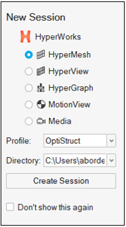
In the New Session window, select HyperMesh from the list of tools.
For Profile, select OptiStruct.
Click Create Session.
Figure 2. Create New Session This loads the user profile, including the appropriate template, menus,
and functionalities of HyperMesh relevant for
generating models for OptiStruct.
Import the Model
On the menu bar, select File > Import > Solver Deck.
In the Import File window, navigate to and select
thermal.fem you saved to your
working directory.
Click Open.
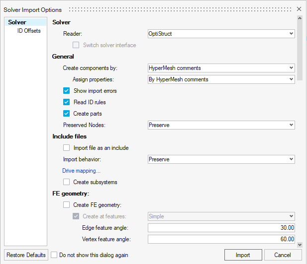
In the Solver Import Options dialog, ensure the Reader is
set to OptiStruct.
Figure 3. Import Base Model in HyperMesh
Accept the default settings and click Import.
Tip: Alternatively, you can drag and drop the file from your file
browser into the application window to open the model file.
Set Up the Model
Create the Thermal Material Properties
In the Model Browser, right-click and select Create > Material.
A default MAT1 material displays in a
Create Material window.
For Name, enter steel.
Select the check box next to MAT4.
The MAT4 card image appears below
MAT1 in the material information area. The
MAT1 card defines the isotropic structural material. The
MAT4 card is for the constant thermal material.
MAT4 uses the same material ID as
MAT1.
In the Create Material window, enter the following values
for the material, steel:
[E] Young’s modulus = 2.1 x 10¹¹ Pa
[NU] Poisson’s ratio = 0.3
[RHO] Material density = 7.9 x 10³ Kg/m3
[A] Thermal expansion coefficient = 1 x 10⁻⁵ / °C
[K] Thermal conductivity = 73W / (m * °C)
[H] Heat transfer coefficient = 40W / m2 °C
Figure 4. Material Entity Editor
Click Close.
A new material, steel, is created with both structural and thermal
properties.
In the Model Browser, right-click and select Create > Property.
A default PSHELL property displays in a
Create Property window.
For Name, enter solid.
For Card Image, select PSOLID from the drop-down
menu.
For Material, click Unspecified.
Click .
In the Advanced Selection window, select
steel and click OK.
Click Close.
The property of the solid steel pipe has been created as 3D PSOLID.
Material information is linked to this property.Figure 5. Assign Material Steel to Property Solid
Link the Material and Property to the Existing Structure
Once the material and property are defined, they need to be linked to the
structure.
In the Model Browser, double click
Components to open the Components Browser.
Click on the pipe component.
The component template displays in the Entity Editor.
For Property, click Unspecified.
Click .
In the Advanced Selection window, select
solid and click OK.
Figure 6. Assign Material and Property
Apply Thermal Loads and Boundary Conditions
In this exercise, the thermal boundary conditions are applied on the
model and saved in a predefined load collector spc_temp. A predefined node 4679
specifies the ambient temperature. A predefined node set node_temp contains the
nodes on the inside surface of the pipe.
Create Temperatures on the Inner Surface of the Pipe
In the Model Browser, double-click Load
Collectors.
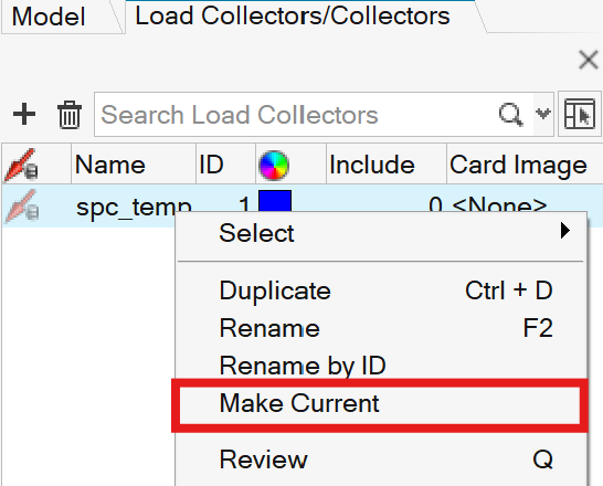
In the browser tab, right-click spc_temp and select
Make Current from the context menu.
Figure 7. Make spc_temp Load Collector Current
From the Analyze ribbon, select Constraints.
Figure 8. Add Constraints
For Entities, select Nodes > .
In the Advanced Selection window, select By
Set from the drop-down menu.
Select node_temp and click
OK.
Figure 9. Advanced Selection Menu
Clear the check boxes for DOF1,
DOF2, DOF3,
DOF4, DOF5, and
DOF6.
For Load Type, select SPC.
Click Create and Close.
This applies the temperature 0.0 on the inside nodes. In the next step,
the temperature value is updated to 60.Figure 10. Create Constraints
In the Model Browser, in Loads, double-click
SPC.
Right-click and choose Select > All from the context menu.
For D, enter 60.0.
Figure 11. Temperature Update
Create Ambient Temperature
From the Analyze ribbon, Thermal tool group, select
Temperatures.
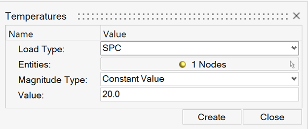
Figure 12. Add Temperature
For Entities, select Nodes > .
In the Advanced Selection window, select By
ID from the drop-down menu.
In the text box, enter 4679 and click
OK.
Figure 13. Advanced Selection Menu
For Load type, select SPC.
For Value, enter 20.
Click Create and Close.
Node 4679 is highlighted.Figure 14. Ambient Temperature Update
Create Heat Convection Surfaces
From the Analyze ribbon, select Convection.
Figure 15. Select Convection
For Type, select Convection from the drop-down
menu.
For ELSETID, select > Create.
Figure 16. Creating ELSETID
For Elements, select Faces from the drop-down
menu.
In the Advanced Selection dialog, select By
ID from the drop-down menu and enter ID
4679.
Figure 18. Create Convection
Click Close.
Create a Heat Transfer Load Step
An OptiStruct steady state heat convection load step is
created, which references the thermal boundary conditions in the load collector
spc_temp. The gradient, flux, and temperature output for the heat transfer analysis
is also requested.
In the Model Browser, right-click and select Create > Load Step.
For Name, enter heat_transfer.
For Analysis type, select Heat transfer (steady state)
from the drop-down menu.
For SPC, click to open Advanced Selection.
Select spc_temp and click
OK.
Select the Output check box.
Under Output, select the FLUX and
THERMAL check boxes.
For both outputs, for FORMAT select H3D.
For both outputs, for OPTION select ALL.
Click Close.
Submit the Job
Run OptiStruct.
From the Analyze ribbon, click Run OptiStruct
Solver.
Figure 19. Select Run OptiStruct Solver
Select the directory where you want to write the OptiStruct model file.
For File name, enter thermal_complete.
The .fem filename extension is the recommended extension
for Bulk Data Format input decks.
Click Save.
Click Export.
For run options, toggle analysis.
In the Altair Compute Console, click
Run.
If the job is successful, an "OptiStruct Job Completed" message appears
in the Compute Console Solver View Message Log. New results
files are in the directory where the model file was written. The
thermal_complete.out file is a good
place to look for error messages that could help debug the input deck if any
errors are present.
View the Results for Heat Transfer Analysis
A "Process completed successfully" message appears in the HyperWorks Solver
View window.
In the HyperWorks Solver View window, click
HyperView.
HyperView is launched and the results are
loaded. A message window appears to inform model and results files were
successfully loaded.
Close the message window, if one appears.
Click Contour .
Figure 20.
In the first pull-down menu below Result type, select Grid
Temperatures (s).
Click Apply.
A contour plot of grid temperatures is created. You may have to use the
Edit Legend function to get the contour.
In the first pull-down menu below Result type, select Element Fluxes
(V).
Click Apply.
A contour plot of fluxes is created. You may have to use the Edit Legend
function to get the contour.Figure 21. Grid Temperatures Contour Plot Figure 22. Element Fluxes Contour Plot



 .
.


 Constraints.




 Convection.

 > Create.





