MacNeal-Harder TestThe patch test is a classical
benchmark problem for the element. If it produces correct results for the test, the result
for any problem solved with the element will converge toward the correct solution. The
intended purpose of the proposed problem set is to ascertain the accuracy of finite element
in various applications.
Model Files
Before you begin, copy the file(s) used in this problem
to your working directory.
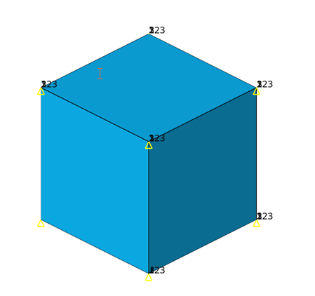
The outer dimension have a unit cube of 1 mm size. There is a mesh of the cube with
node locations as mentioned in the table with first order CHEXA elements. The eight
corners of the cube are constrained in all three translational direction and free in
all three rotational directions. Displacement is enforced using
SPCD on the eight nodes of cylinder in X, Y and Z translation
directions of the cube.
The material properties are:
Material Properties
Value
Young's Modulus
1 x 10⁶ Pa
Poisson's Ratio
0.25
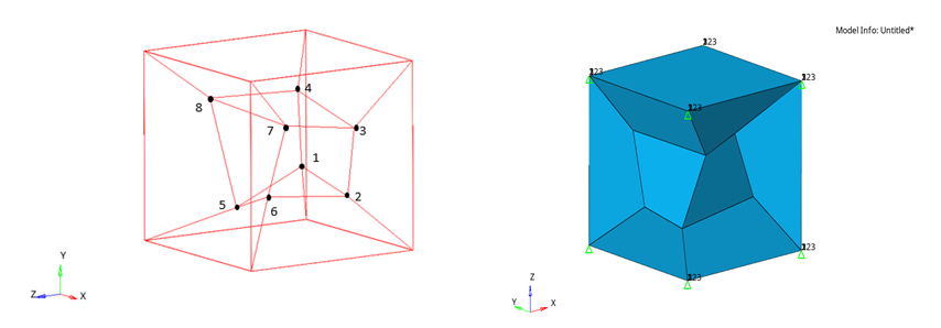
Figure 2. Patch test for solids
Table 1. Location of Inner Nodes
x
y
z
1
0.249
0.342
0.192
2
0.826
0.288
0.288
3
0.850
0.649
0.263
4
0.273
0.750
0.230
5
0.320
0.186
0.643
6
0.677
0.305
0.683
7
0.788
0.693
0.644
8
0.165
0.745
0.702
The arbitrarily distorted element shapes are an essential part of the test. The
principal virtue of a patch test is that if an element produces correct results for
the test, the results for any problem solved with the element will converge toward
the correct solution as the elements are subdivided. On the other hand, passing the
patch test does not guarantee satisfactory results, since the rate of convergence
may be too slow for practical use. The above patch test is an extension of
Robinson’s patch test to three dimensions.
Displacement boundary conditions for the test are:
u
v
w
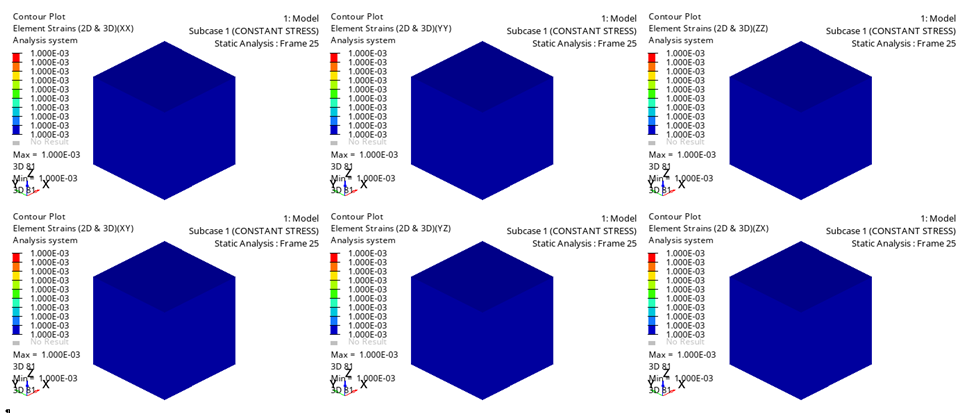
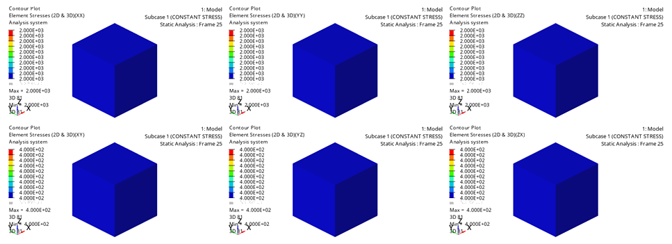
Results
Figure 3. Elemental strains in all 6 direction plot Figure 4. Elemental stresses in all 6 direction plot
The results CHEXA elements agree with the reference results.
Reference
MacNeal, R.H., and Harder, R.L., A Proposed Standard Set of Problems to Test Finite
Element Accuracy, Finite Elements in Analysis and Design, 1 (1985) 3-20