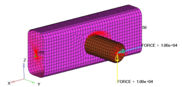
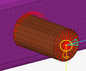
The structural model with loads and constraints applied is shown in Figure 1. The deflection at the end of the tubular cross-member should be limited. The
optimal solution uses as little material as possible.Figure 1. Structural Model of Rail Joint
The structural model is loaded into HyperMesh. The
constraints, loads, material properties, and subcases (loadsteps) are already
defined in the model. Size design variables and optimization parameters are defined,
and OptiStruct determines the optimal gauges for the
components. The results are then reviewed in HyperView.
The optimization problem for this tutorial is stated as:
Objective
Minimize volume.
Constraints
A given maximum nodal displacement at the loading grid point for two
loading conditions.
Design Variables
Gauges of the two parts.
The following exercises are included:
Set up a size optimization in HyperMesh.
Post-process size optimization results in HyperView.
Launch HyperMesh
Launch HyperMesh.
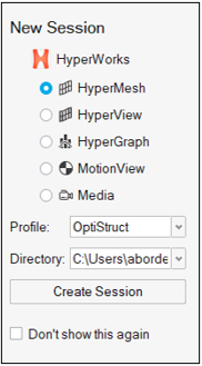
In the New Session window, select HyperMesh from the list of tools.
For Profile, select OptiStruct.
Click Create Session.
Figure 2. Create New Session This loads the user profile, including the appropriate template, menus,
and functionalities of HyperMesh relevant for
generating models for OptiStruct.
Open the Model File
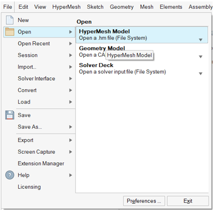
On the menu bar, select File > Open > HyperMesh Model.
Navigate to and select the joint_size.hm file saved in your
working directory.
Click Open.
The joint_size.hm database is loaded into the current
HyperMesh session, replacing any existing
data.Figure 3. Model Import Options
Tip: Alternatively, you can drag and drop the file onto the
viewport from the file browser window.
Set Up the Model
Create Size Design Variables
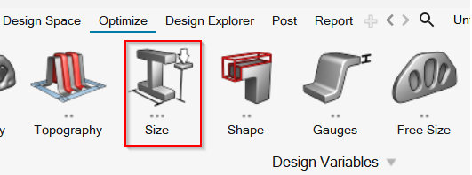
Open the Optimize ribbon.
Under Design Variables, click Size.
Figure 4. Size
For Name, enter tube.
For Move Limit, enter 0.1.
Click initial value and enter
1.0.
Click lower bound and enter
0.1.
Click upper bound and enter
5.0.
Click Close.
A design variable, tube, has been created. The design variable has an
initial value of 1.0, a lower bound of 0.1, and an upper bound of
5.0.
Repeat steps 1 through 8 to create the design variable named rail using the
same move limit, initial value, lower, and upper bounds.
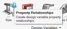
In the Size tool group, click the Property Relationships
satellite icon.
Figure 5.
For Name, enter tube_th.
For Property ID, click Unspecified.
Click the Search tool.
Select tube.
For the List of Design Variables, select
Designvars.
Click to open Design Variables Advanced Selection.
Select tube and click OK.
Click Close.
A design variable to property relationship, tube_th, has been created
relating the design variable tube to the thickness entry on the
PSHELL card for the property tube.
Repeat steps 10 through 18 to create the design variable to property relationship
rail_th relating the design variable rail to the
thickness entry on the PSHELL card for the property
rail.
Create Responses
For more details, see the OptiStructResponses
User Guide.
On the Optimize ribbon, Targets tool group, click
Responses.
Figure 6. Responses
For Name, enter volume.
For Response type, select volume.
Verify the Property Type is set to total.
Click Close.
A response, volume, is defined for the total volume of the
model.
Click the Responses tool to create another
response.
For Name, enter X_Disp.
For Response type, select static displacement.
For List of Nodes, click 0 Nodes to start selecting,
then choose the node at the center of the rigid spider at the loading point
(node 3143).
Figure 7. Select Node
Click the check mark.
Select DOF1.
Click Close.
A response, X_Disp, is defined for the x-displacement of the node
3143.
Similarly, create another Response named Z_Disp.
For Response type, select static displacement.
For List of Nodes, click 0 Nodes to start selecting,
then choose the node at the center of the rigid spider at the loading point
(node 3143).
Click the check mark.
Select DOF3 and click
Close.
A response, Z_Disp, is defined for the z-displacement of the node
3143.
Create Constraints
A response defined as the objective cannot be constrained. In this case, you cannot
constrain the response volume.
Upper bound constraints are to be defined for the responses X_Disp and Z_Disp.
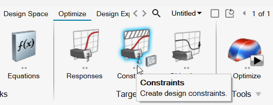
On the Optimize ribbon, Targets tool group, click
Constraints.
Figure 8. Constraints
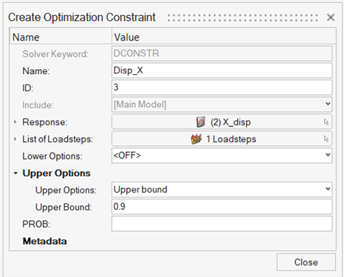
For Name, enter Disp_X.
For Response, select Unspecified.
Click the Search tool and select
X_Disp.
For List of Loadsteps, click 0 Loadsteps > to open Advanced Selection.
Select FORCE_X.
Click OK.
For Upper Options, select Upper bound from the
drop-down.
For Upper Bound, enter 0.9.
Figure 9. Create Disp_X Optimization Constraint
Click Close.
A constraint is defined on the response X_Disp. The constraint is an
upper bound with a value of 0.9. The constraint applies to the subcase
FORCE_X.
Similarly, repeat steps 1 through 10 to create another Constraint named Disp_Z with:
Response: Z_Disp
Loadstep: FORCE_Z
Upper Bound: 1.6
Figure 10. Create Disp_Z Optimization Constraint
Define the Objective Function
In this example, the objective is to minimize the volume response defined
previously.
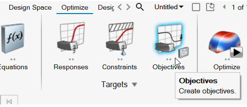
On the Optimize ribbon, Targets tool group, click
Objectives.
Figure 11. Objectives
Verify the Objective Type is set to Minimize.
For Response, click Unspecified.
Click the Search tool and select
volume.
Click Close.
The objective function is now defined.
Save the HyperMesh Database
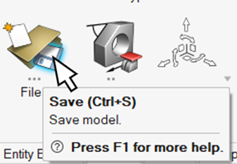
From the ribbon, File tool group, select the Save.hm file icon.
Figure 12. Save
Select the directory where you would like to save the database.
For File name, enter joint_sizeOPT.hm.
Click Save.
Run the Optimization
From the Optimize tool, click Run.
Figure 13. Run Optimization
Select the directory where you want to write the OptiStruct model file.
For File name, enter joint_sizeOPT.
The .fem filename extension is the recommended extension
for Bulk Data Format input decks.
Click Save.
For Export, select All.
Click Export.
In the Altair Compute Console, click
Run.
If the job is successful, new results files are seen in the directory
where the model file was written. The joint_sizeOPT.out file is a good place to look for error messages that could
help debug the input deck if any errors are present.
Important
files for the size optimization include:
joint_sizeOPT.hgdata
file containing data for
the objective function, percent constraint violations, and
constraint for each iteration.
joint_sizeOPT.prop
OptiStruct property output file
containing all updated property data from the last iteration for
size optimization.
joint_sizeOPT.hist
OptiStruct iteration history file
containing the iteration history of the objective function and
of the most violated constraint. This file can be used for a xy
plot of the iteration history.
joint_sizeOPT.out
OptiStruct output file containing
specific information on the file setup, the setup of the
optimization problem, estimates for the amount of RAM and disk
space required for the run, information for all optimization
iterations, and compute time information. This file contains
compliance, volume calculations, and gauge information for
optimization iterations. It is highly recommended to review this
file for warnings and errors.
joint_sizeOPT.res
HyperMesh binary result file.
joint_sizeOPT_des.h3d
HyperView binary result file
containing the design iteration results.
joint_sizeOPT_s1.h3d
HyperView binary result file
containing the analysis results of subcase with ID 1.
joint_sizeOPT_s2.h3d
HyperView binary result file
containing the analysis results of subcase with ID 2.
joint_sizeOPT.stat
Summary of analysis process, providing CPU information for each
step during analysis process.
Post-process the Results
Displacement and stress results are output by default for linear
static analyses. This section describes how to view those results in HyperView. Size optimization results from OptiStruct are given in the .h3d files
and joint_sizeOPT.out.
joint_sizeOPT_des.h3d
Contains the element thickness for all five iterations.
joint_sizeOPT_s1.h3d
Contains displacement and stress results for the linear static analysis
for iteration 0 and iteration 4 of the subcase with ID 1 (subcase
Force_X).
joint_sizeOPT_s2.h3d
Contains displacement and stress results for the linear static analysis
for iteration 0 and iteration 4 of the subcase with ID 2 (subcase
Force_Z).
joint_sizeOPT.out
Contains gauge and volume information for all iterations.
The results contained in the HyperView binary
results are examined first. Then the gauge history in the
joint_sizeOPT.out file are also reviewed.
View the Size Optimization Results
View the gauge thickness.
When the "OptiStruct job completed" message appears in the Run
Summary window, click Results.
HyperView is launched and
joint_sizeOPT_des.h3d is loaded.
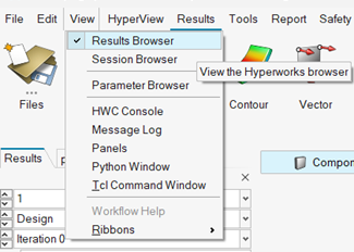
In the Results Browser, select the first iteration.
Note: If the Results Browser is not visible, you can activate it using the View
menu on the menu bar.
Figure 14. View Menu
From the Post ribbon, Plot tool group, click
Contour.
Figure 15.
For Results type, ensure the first drop-down is set to Element
Thicknesses (s).
Ensure the second drop-down is set to Thickness.
Verify Averaging method is set to None.
Click Apply.
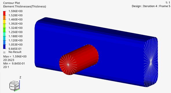
In the Results Browser, select the last iteration.
A contoured image representing shell thickness should be visible. Each
element in the model is assigned a legend color, indicating the thickness value
for that element for the current iteration.Figure 16. Thickness Contour at Last Iteration
View the Displacement Results
It is helpful to view the deformations of the model to determine if the boundary
conditions have been met and to see if the model is deforming as expected.
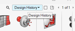
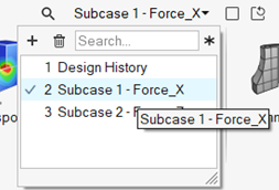
In HyperView, click Design
History to expand the Page Selection
dialog.
Figure 17. Design History
Select Subcase 1-Force_X.
Figure 18. Select Subcase
Note: If the other pages are not available in the drop-down menu:
Click File > Session > Open.
Select joint_sizeOPT.mvw.
Click Open.
Click Yes.
Now the other options should be available in the drop-down.
From the Post ribbon, Plot tool group, click
Contour.
Figure 19.
For Results type, in the first drop-down menu, select Displacement
[v].
In the second drop-down menu, select X.
Verify Averaging method is set to None.
Click Apply.
The resulting contours represent the x component displacement field
resulting from the applied loads and boundary conditions.
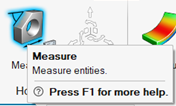
In the Home tool group, select Measure.
Figure 20. Measure Tool
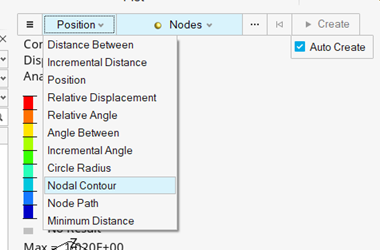
From the first drop-down menu on the guide bar, select Nodal
Contour.
Figure 21. Select Nodal Contour
Click Nodes and select the rigid spider node with loads
(node 3143).
Figure 22. Displacement on X-Direction for the X-Force Loadcase at the First
Iteration The x-displacement value for 3143 (center of rigid spider, where loading
is applied) is shown in the modeling window. The
x-displacement is larger than the upper bound constraint of 0.9 that you defined
earlier.
In the Results Browser, select the last iteration.
Figure 23. Displacement on X-Direction for the X-Force Loadcase at the Last
Iteration The contour now shows the x-displacement results for Subcase 1 (FORCE_X)
and iteration 4, which corresponds to the end of the optimization iterations.
The x-displacement is now less than 0.9.
Expand the Page Selection dialogue and select
Subcase 2-Force_Z.
Note: The name of the page is displayed as Subcase 2 – Force_Z to indicate that
the results correspond to subcase 2.
From the Post ribbon, Plot tool group, click
Contour.
Figure 24.
For Results type, in the first drop-down menu, select Displacement
[v].
In the second drop-down menu, select Z.
Click Apply.
Repeat steps 8 through 11 to measure and display the z-displacement value for node 3143.
Figure 25. Displacement on Z-Direction for the Z-Force
Loadcase, First Iteration
Figure 26. Displacement on Z-Direction for the Z-Force
Loadcase, Last Iteration
Alternate Method to View Gauge Thickness Results
From the UNIX or MSDOS shell, open the joint_sizeOPT.out
file in a text editor.
Review all five iterations, noting the volume, constraint information, and
gauge at each iteration.
Has the volume been minimized for the given constraints?
Have the displacement constraints been met?
What are the resulting gauges for the rail and tube?

 Search tool.
 to open Design Variables Advanced Selection.

 check mark.