Tutorial Level: Intermediate In this tutorial you will learn how to setup an optimization problem using MotionView’s Optimization Wizard.
MotionSolve is commonly used for performing system level
simulation. Simulations are commonly performed to understand how well a specific
design performs. Often a goal for such simulations is to find the right set of
design parameters that permit the system to perform its intended functions in some
optimal way.
Commonly used design variables are the location and orientation of various connectors
and their force characteristics. Occasionally the mass and material properties of
some bodies are also included as design variables. The system behavior is normally
characterized with a set of response variables. So, the goal of simulations often is
to find the values of these design variables such that the response variables attain
a desired set of values.
In the past such analysis has been done using techniques such as Monte Carlo
simulations and design of experiments. These methods work quite well, but they are
computationally intensive and require large sets of simulations.
MotionSolve now supports a capability for analytically computing design
sensitivities. Design sensitivity is the matrix of partial derivatives of the
response variables with respect to the design variables. A gradient-based optimizer
is capable of using these sensitivities to minimize a cost function. This process is
known as design optimization. A new optimization toolkit that permits optimization
of some design problems is also now available in MotionSolve.
Though not as general as the statistical methods, optimization with design
sensitivity is significantly faster and is the preferred solution in many
instances.
In this tutorial you will learn about the following:
Process of Optimization with MotionSolve
Defining spring stiffnesses as design variables
Defining displacements as responses
Using the responses as objectives
Running the optimization and post-processing the results
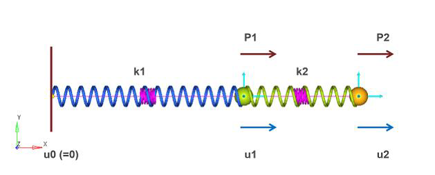
Introduction
Two springs are connected in series. The stiffness of spring-1 is k1 and
that of spring-2 is k2. One end of spring-1 is fixed to ground while a
force, P1, acts at the other end. Spring-2 is subjected to a force of P2
at the other end.
The objective of the analysis is to determine the sensitivities of
stiffnesses of the springs to displacements u1 and u2 and use them to
identify or tune k1 and k2 of the system to achieve specific values of
u1 and u2.
MotionSolve's DSA (Design Sensitivity Analysis) capability to calculate
sensitivities is utilized in this example. A Step-by-step procedure to
define and run the model is given in the tutorial.
Figure 1 shows that
problem setup. Properties used in the problem are also provided. Figure 1. Springs in Series – Model Description
A list of properties for the system follows:
Displacement: u0 =0 (Fixed)
Force:
P1 = 1N
P2 = 2N
Stiffness:
k1 = 2 N/mm
k2 = 3 N/mm
Response Variables (RV): u1 and u2
Design Variables (DV): k1 and k2
Analysis Type: Static Analysis with DSA
The process of optimization starts with setting up a model in MotionView. MotionView’s
Optimization Wizard is used to setup design variables, responses and objectives. The
wizard also guides the user to run and plot/print results of optimization. It is
also able to export a design from a particular iteration into a new MDL for further
analyses.
Add Design Variables
In this step, you will add design variables for the optimization.
Before you begin, copy the file
mv_3020_initial_two_springs.mdl located in the
mbd_modeling\motionsolve\optimization\MV-3020 into your
<working directory>.
Open mv_3020_initial_two_springs.mdl in MotionView.
In the Project Browser, right-click on
Model and select Optimization
Wizard from the context menu.
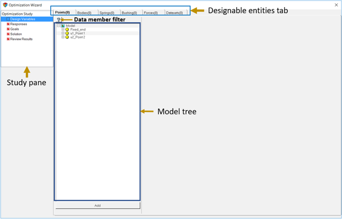
This will display the Optimization Wizard.Figure 2. The wizard consists of an Optimization Study pane that guides the user
through each step of solving an optimization problem with MotionSolve. The wizard opens with the Design
Variables page active that enables the selection of design
variables.
Under Design Variables, click on the Springs tab.
Two SpringDampers will be listed:
K1_SpringDamper
K2_SpringDamper
The spring stiffness of these springs are made designable.
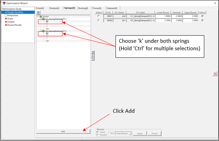
Expand the two springs by clicking on the ‘+’
button.
The data members that can be made designable are displayed as in Figure 3:Figure 3. Spring data members that can be made as designable
Using the Control keyboard button, select the
k (stiffness) data members of both the springs. Click
the Add button available at the bottom of the Model Tree.
The stiffness of SpringDampers are added as design variables with
default upper and lower bound. The default value used by MotionView for calculating bounds is 10% of nominal
value.
Modify the upper and lower bounds for stiffness as shown in Table 1:
Table 1.
DV
Lower Bound
Upper Bound
sd_0.k
0.25
4.0
sd_1.k
0.25
4.0
Note: The number within parenthesis of the designable entities tab at
the top (Springs(2) in this case) indicates the number of design variables
defined of that entity type.
You have now finished defining design
variables.
Add Response Variables
In this step, you will add response variables for the optimization.
There are two responses in this problem:
Displacement u1: To make u1 to reach a value of 3, the metric (1-u1/3)**2 is
used.
Displacement u2: To make u2 to reach a value of 4, the metric (1-u2/4)**2 is
used.
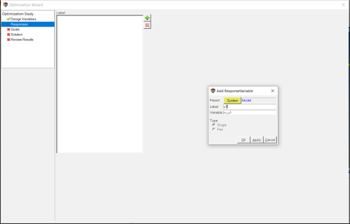
Click on the Responses page.
Click to add a response variable. In the dialog that appears,
change the Label to u1 and click OK.
Figure 4. Adding response1 – u1 The ResponseVariable is added and appears in the list. The panel also
appears.
In the panel, use the combo box to change the Response Type to
Generic.
Accept the default value of 1.0 for the scale.
In the Response Expression key, enter the following expression:
`(1-DM({b_0.cm.id},{m_0.id})/3)**2`
Where:
b_0.cm.id = ID of the CM marker of Body 0
m_0.id = ID of the marker on ground body located at u1_Point 1
Note: During optimization, the optimizer tries to minimize the entire expression
and as the value of DM({b_0.cm.id},{m_0.id}) approaches 3, the value of this
response is minimized.
Check on the Use derivative check box.
When checked, the computed value of the expression at the last time step
of the simulation is used as the response.
Repeat the steps above to add another ResponseVariable
u2 with the following specifications:
The objectives are as follows: the value of u1 should be 3 and value of u2 should
be 4 at the end of optimization. You can use the responses you created in the previous
section as objectives.
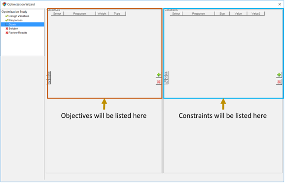
Navigate to the Goals page.
This page has two sections: Objectives and Constraints.Figure 5.
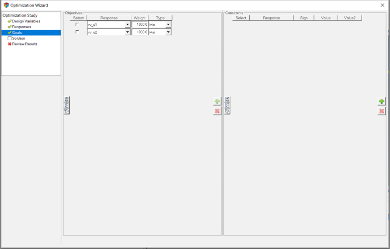
Under Objectives, click the button.
This will add an objective with the response rv_u1.
Change the Weight to 1000. Retain the Type as
Min in order to minimize the response.
Repeat steps 2
and 3 to add a
second objective (rv_u2).
Figure 6. Defining objectives There are no constraints in this problem. You have completed model
setup.
Run the Optimization
In this step you will run the optimization.
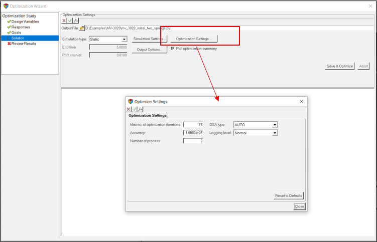
Navigate to the Solutions page to specify optimization
settings and run the analysis.
Note: The model is saved before running, and if this is not desired, the model
can be saved with a different mdl file name before starting the
optimization. This can be done by closing the wizard, saving the model with
a different name and returning to the wizard again.
Click on the Optimization Settings button. In the
Optimizer Settings dialog that appears, change Accuracy to
1.0e-5.
Figure 7. Optimization settings for this problem
Retain the rest of the parameters with default values.
Close the dialog.
Click on Save & Optimize to start the
optimization.
While the optimization is running, a plot of total weighted cost vs.
iteration number and a plot of individual cost vs. iteration number are
displayed in a separate window (after the initial simulation).
Once the
optimization is complete a summary is listed in the text
window.
Note: You may have to scroll down to the end and/or to the right
to see results of the optimization.
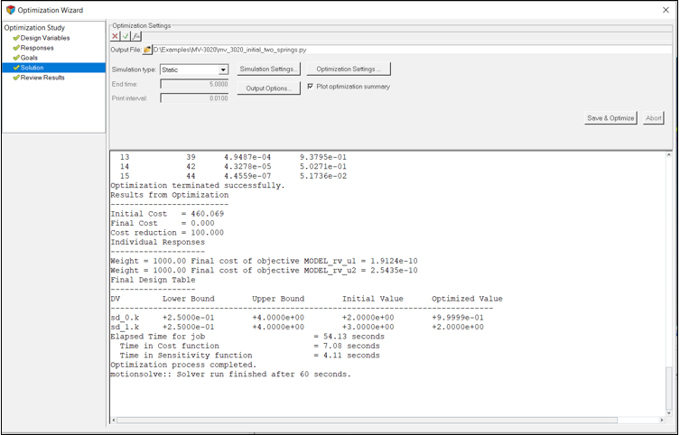
The text window should appear as
in Figure 8:Figure 8. Text window after the optimization is complete
The following list shows important information available in the output
window:
Optimizer settings
Iteration summary - Value of cost function by iteration number
Results from optimization - Initial cost, final cost and percentage
reduction in cost
Final value of each objective at the end of optimization
Final design table with information on design variable bounds and
initial and optimized values of design variables
Elapsed time for calculating cost and sensitivity
Post-Process
In this step, you will post-process the results of optimization.
MotionView provides the ability to list, plot and
animate results of optimization. It also provides capability to export mdl model
corresponding to any design iteration.
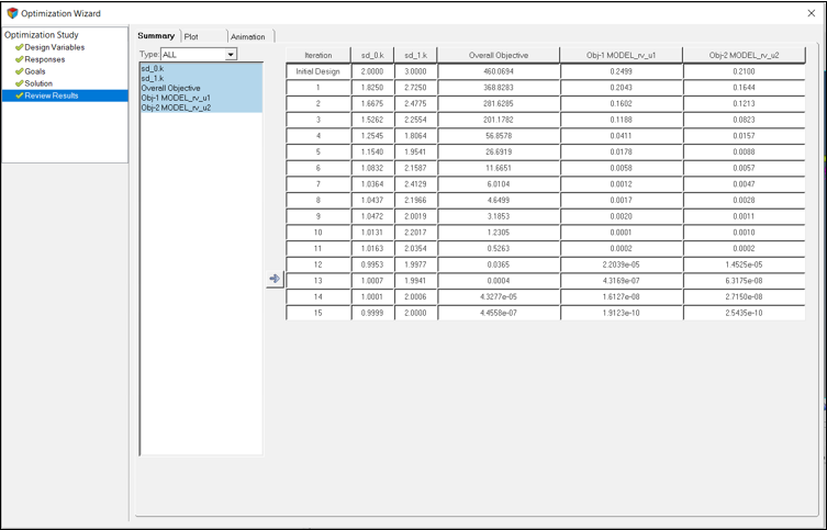
Navigate to the Review Results page.
The Summary tab appears that lists the history of design variables,
responses and objective functions in a tabular format for each iteration of
optimization run.
Note:MotionSolve uses SLSQP
algorithm for optimization. Hence the last iteration is usually the optimum
configuration with least value of cost function. See Figure 9. Figure 9. Summary tab listing cost function (objective), response variables
and design variables
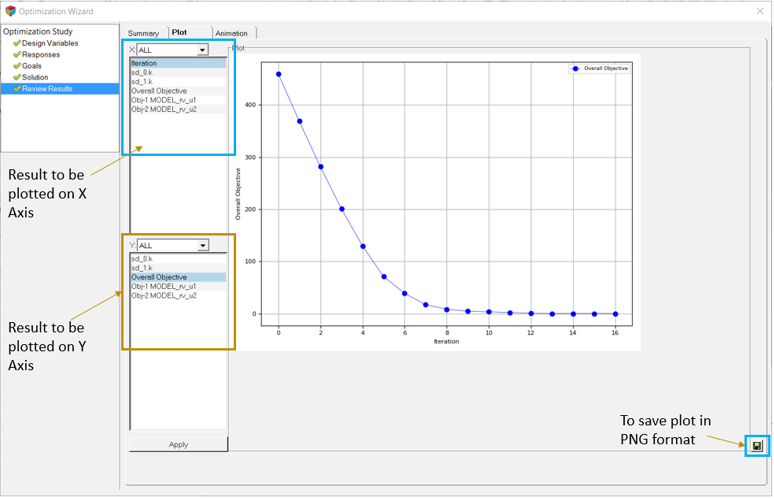
Click the Plot tab.
It helps to visualize a variation of design variables, response variables and
cost function using graphs. You can choose to plot any number of variables along
the y-axis with respect to a variable along the x-axis.Figure 10.
Select Iteration from the X list and Overall
Objective from the Y list. Then click Apply.
Note: You can select and plot multiple items from the Y list.
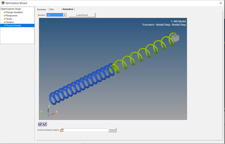
Select the Animation tab to animate the configuration
generated during any iteration.
Load the results file from the last iteration (iteration 16).
In the Iteration drop-down menu, choose
16.
Click Load Result.
The animation is loaded in the display area.
Click (Play).
Since this is a statistic analysis, the animation only has one
frame.Figure 11. Animation tab in the ‘Post Processing’ page The Archive Model location browser is available in this tab for
exporting the model in MDL format from any iteration.
Export the model.
Choose a file path.
Click Export.
This will create an archive folder which contains an MDL and all
other reference files (if any) to run the model. The design variable
values are set to the values in the iteration number you
choose.

 to add a response variable. In the dialog that appears,
change the Label to u1 and click OK.
to add a response variable. In the dialog that appears,
change the Label to u1 and click OK.
 (Play).
Since this is a statistic analysis, the animation only has one frame.
(Play).
Since this is a statistic analysis, the animation only has one frame.