MV-1032: Build Models and Simulations Using Wizards
Tutorial Level: Intermediate In
this tutorial, you will learn how to build a model using the Assembly and Task Wizards in MotionView, how to view a
standard report, and how to modify a model and compare results using the Report
Template.
Model Wizards are powerful tools in MotionView that can be used to quickly build models with standard
topology that is used repeatedly. There are two standard wizards available: the Assembly
Wizard and the Task Wizard (which work in conjunction with one another). Both of these
wizards rely on a library of pre-saved system, analysis, and report definition files to
automate the processes of building models, analyzing them, and post-processing the
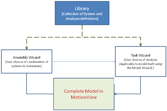
results. The wizard mechanics are shown in Figure 1:Figure 1.
A collection of systems and analyses are stored as a library.
The Assembly Wizard presents the user with various options for selecting systems
to instantiate (in the form of a series of panels).
The systems selected by the user in the panels are instantiated using the system
definitions contained in the MotionView client
library, thereby assembling the model comprised of different systems. An
Attachment Wizard is used to select possible attachment options for each
instantiated system.
Once the model is built, the Task Wizard is invoked in order to attach
applicable events to the model. The selected analysis is instantiated using the
analysis definition stored in the library.
Build a Front Suspension Model using Assembly Wizard
In this exercise, you will build a suspension model of a vehicle using the standard
wizard library available in MotionView.
Start a new MotionView session.
On the menu bar, click Model > Assembly Wizard.
This will display the Assembly Wizard
dialog.
For Model type, click Front end of vehicle. Then click
Next.
For Drive type, click Front Wheel Drive. Then click
Next.
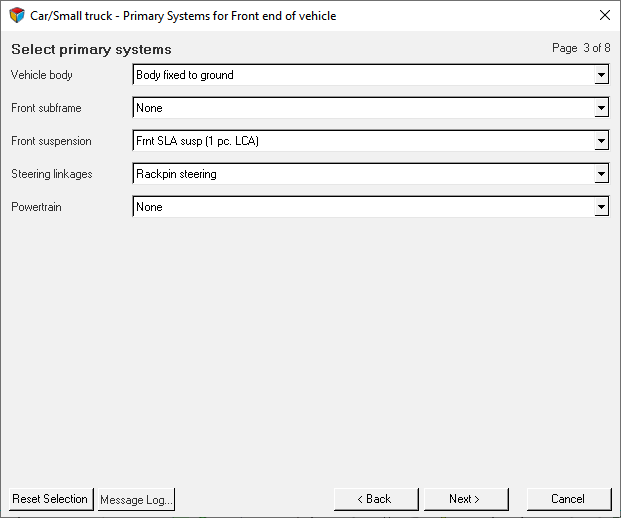
For Primary Systems for Front end of vehicle, make the
selections shown in Figure 2. Then click Next.
Figure 2.
From Select steering subsystems, for Steering Column
choose Steering column 1 (not for abaqus). For Steering
Boost choose None.
Click Next.
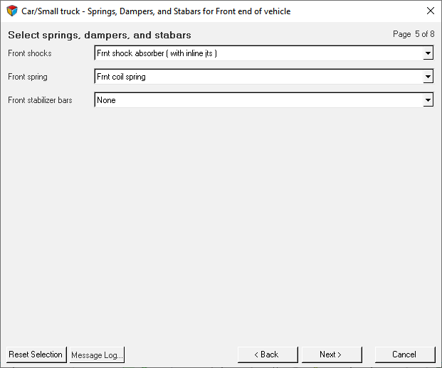
From Select springs, dampers, and stabilizer bars, specify
the options shown in Figure 3. Then click Next.
Figure 3.
From Select jounce and rebound bumpers, choose
None for both options. Then click
Next.
From the Select Driveline Systems dialog, for Front
Driveline choose Independent fwd and click
Next.
You now have all of the required systems for the model. The Next button
is now the Attachments button.
Click the Attachments button to open the
Attachment Wizard dialog.
The Attachment Wizard shows the attachment choices which are available for
each sub-system.
Review and accept the default selections in the Attachment Wizard.
Click Finish.
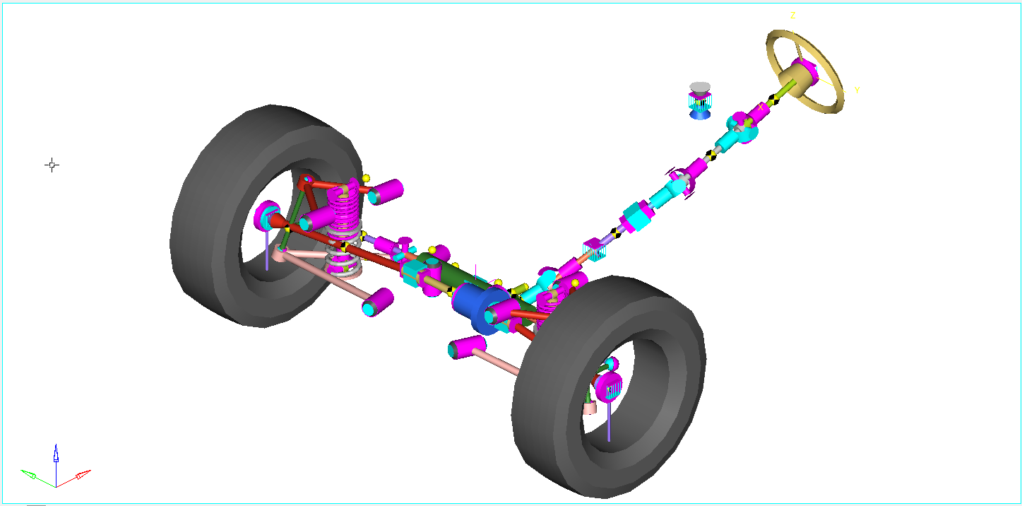
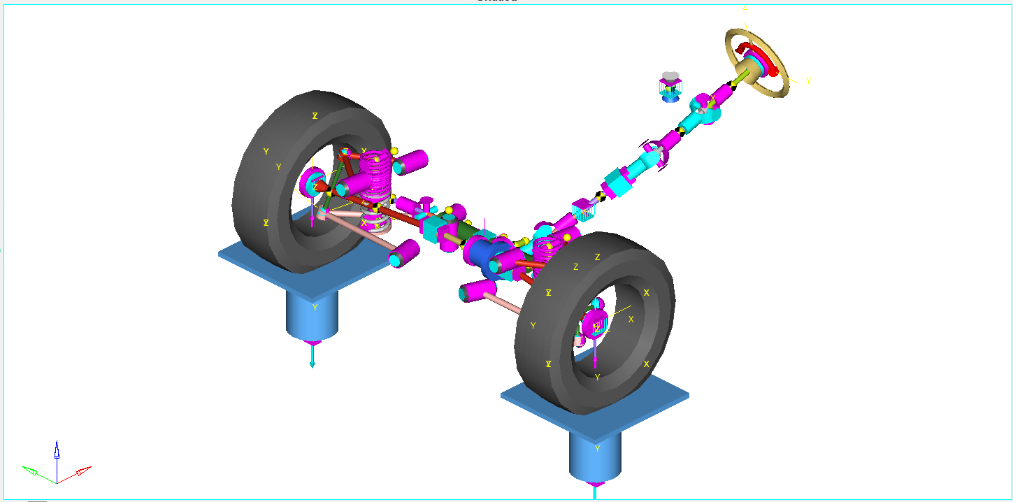
Your model will look like the example in Figure 4: Figure 4. This model represents a front end suspension of a vehicle with a Short
Long Arm type (also known as Wishbone) of suspension and a steering system. The
vehicle body is fixed to ground. The upper and lower control arms of the
suspension are attached to the vehicle body at one end through bushings, while
they are connected to a knuckle on the other end through ball joints. A wheel
hub (no graphics for this body are in the model) is mounted on the knuckle
through a revolute joint. The wheel is fixed to the wheel hub.
The steering system consists of a rack with a translation joint with a rack
housing (through a dummy body). The ends of the rack are connected to a tie rod
at each end through ball joints and the other end of the tie rod is connected to
the steer arm of the knuckle through ball joints. The rack gets its movement
from the steering column through a coupler constraint between the rack and the
pinion.
Add a Static Ride Analysis Task using Task Wizard
In this step you will attach a static ride analysis for the suspension assembly using
the Task Wizard.
The Analysis Task Wizard allows you to assign an event analysis to the model using
a wizard. This default suspension wizard is configured such that the available analyses
choices are dependent on the system selections made in the Assembly Wizard. Since this
is a half-vehicle model, only events that are applicable for a half-vehicle model are
available. Through the analysis you will complete in this step, you can study the
kinematic characteristic of the suspension for varying vertical positions of the wheels.
Both wheels are exercised such that they move vertically along the same
direction.
On the menu bar, click Analysis > Task Wizard.
In the Car/small truck - Front end tasks dialog, from the
drop-down menu select Static Ride Analysis. Then click
Next.
Read the information in the dialog box and click
Finish.
In the Vehicle Parameters dialog, retain the current
parameters and click Finish.
Your model should appear similar to the one shown in Figure 5. The Model Tree in the Project Browser now
includes an Analysis called Static ride analysis. Figure 5.
Note: The static ride analysis event consists of a pair of
jacks that are attached to the wheels at the tire contact patch location.
The jacks are actuated through Actuator Forces that exercises them in the
vertical direction in a sinusoidal fashion. It is possible to add many
different analysis tasks to the same model, however only one analysis task
may be active at one time.
Rename the model My Front SLA Suspension by doing one of
the following:
In the Project Browser, right-click on
Model and select Change
Label from the context menu.
Left-click on Model and press F2 on the keyboard.
In the Project Browser, expand the folders Static ride analysis > Forms and select the Static Ride Parameters
form.
In the Forms panel, for both Jounce travel (mm) and Rebound travel (mm), enter
a value of 50.0.
Click (Save) and save the model as
sla_ride.mdl to your <working
directory>.
Run the Simulation and View the Report
In this step you will run the front suspension model simulation and view the standard
report.
The static ride simulation is a 10 second quasi-static run. Within the 10 seconds
the jack moves in jounce (vertically upwards), then moves down until the rebound
position is reached (distance from the initial position downwards), and then back to its
initial position. The amount of travel is as per the distance specified in the Static
Ride parameters form.
On the General Actions toolbar, click (Run).
Click the and specify the name of the solver file as
sla_ride_baseline.xml.
Save the solver file to your <working directory>.
Click the Run button.
When the job is completed, close the Solver window and
clear the Message Log.
On the menu bar, click Analysis > View Reports.
In the dialog, choose Front Ride-MSolve SDF based Report My Front
SLA Suspension. Then click OK.
This analysis comes with a Standard Report Template that plots the results and
loads the animation in subsequent pages.
Use the and buttons to navigate the plots and animation pages
in the report.
The last page is the TextView client with an open
Suspension Design Factors (SDF) report. This report lists the suspension factors
at each time interval of the simulation.
How does viewing pre-specified results work?
A report that refers to a report template file (a template that
contains plot and animation definitions) can be defined in the
MotionView model using the
*Report() MDL statement. Whenever a model
containing such a report definition is submitted to a solver,
MotionView writes a record of the
report into a log file named .reports. You can
specify the location of this file with the preference file statement
*RegisterReportsLog(path). The default location
of the .reports file is:
UNIX - <user home>
PC - C:\Documents and
Settings\<user>
You can also set the path of the
.reports file by selecting the Set
Wizard path option under the Model menu.
When
View Reports from the Analysis menu
is selected, MotionView displays the
contents of the .reports file in the
Reports dialog. When you select a report from the dialog,
MotionView loads the requested
report definition file into your session.
The following is
a sample entry from the .reports log
file:
Front Ride - MSolve Report Front Static Ride
02/10/XX 06:07:58
E:/Altair/hw/mdl/mdllib/Libs/Tasks/adams/Front/Ride/ms_rep_kc_front.tpl
*Report(rep_kc_frnt_mc, Front Ride - MSolve Report, repdef_kc_frnt,
"E:/Temp/sla_rigid.h3d", "E:/Temp/sla_rigid.h3d", "E:/Temp/sla_rigid.plt")
The
first line contains the report label, model label, and the date
and time when the solver input files were saved. This
information is contained in the Reports
dialog. You should give your models specific names, otherwise
they will be labeled Model.
Line 2 contains the name of
the report definition file that the report is to be derived
from.
Line 3 contains an MDL statement called
*Report(). This statement specifies the
report definition variable name along with the required
parameters. Refer to the MDL online help for more
information.
Modify the Model Parameters
In this step you will modify the suspension parameters and re-run the
simulation.
Return to the MotionView client page.
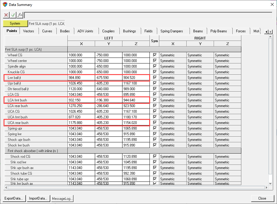
In the Project Browser, right-click on Frnt SLA
susp (1 pc. LCA) and select Data Summary
from the context menu.
This will display the Data Summary dialog. Figure 6.
Append +10 to the Z coordinate of Lwr ball jt.
Change the coordinates for LCA frnt bush.
Append -5 to the X coordinate.
Append +5 to the Y coordinate.
Change the coordinates for the UCA rear bush.
Append +3 to the X coordinate.
Append -5 to the Y coordinate.
Click on the Bushings tab.
Change the KZ value of LCA frnt bush to -200.
Change the KZ value of UCA frnt bush to +200. Then click
Close.
On the General Actions toolbar, click (Run).
Click the and specify the name of the solver file as
sla_rigid_change.xml.
Save the solver file to your <working directory>.
Click the Run button.
When the job is completed, close the Solver window and
clear the Message Log.
Compare Results
In this step, you will compare the reports for both suspension
simulations.
On the menu bar, click Analysis > View Reports.
Click the most recent report (located at the top of the list) and click
OK.
This will overlay the new results in the plot and animation
windows.
Use the and buttons to navigate to the HyperView client page (page 17 of the
session).
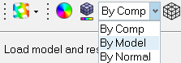
From the toolbar, change the Color Mode to By
Model.
Figure 7.
The visualization of the second overlayed model is now changed.
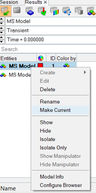
In the Results Browser, go to the Files
View. Make the first Model current
using the right-click context menu as shown in Figure 8.
Figure 8.
Change the Color Mode for this model, following step 4 above.
From the Animation toolbar, click the (Start/Pause Animation) button to animate your results.
Now you can observe the differences between the two models.
Navigate to the MotionView client page.
Click to save the model.
Click (Save Session).
Save the file as my_susp_analysis.mvw in your
<working directory>.
The model, plot, and animation information is saved in the session
file.

 (Save) and save the model as
sla_ride.mdl to your <working
directory>.
(Save) and save the model as
sla_ride.mdl to your <working
directory>.
 (Run).
 and specify the name of the solver file as
sla_ride_baseline.xml.
and specify the name of the solver file as
sla_ride_baseline.xml.
 and
and  buttons to navigate the plots and animation pages
in the report.
The last page is the TextView client with an open Suspension Design Factors (SDF) report. This report lists the suspension factors at each time interval of the simulation.
buttons to navigate the plots and animation pages
in the report.
The last page is the TextView client with an open Suspension Design Factors (SDF) report. This report lists the suspension factors at each time interval of the simulation. MotionView client page.
 HyperView client page (page 17 of the
session).
HyperView client page (page 17 of the
session).
 . Make the first Model current
using the right-click context menu as shown in Figure 8.
. Make the first Model current
using the right-click context menu as shown in Figure 8.
 (Start/Pause Animation) button to animate your results.
Now you can observe the differences between the two models.
(Start/Pause Animation) button to animate your results.
Now you can observe the differences between the two models.
 (Save Session).