Vehicle Wading Simulation
Setup a vehicle wading simulation.
Vehicle Wading Approaches
Another solution type is introduced, designed for simulating vehicle wading through deep water. These simulations are characterized by a complex geometry interacting with a free surface fluid. This is difficult and expensive to capture with traditional CFD approaches, but SPH's Lagrangian method is ideally suited to this kind of problem.
- Moving Vehicle
- This approach mimics a real world condition. A water channel is defined and the vehicle drives through it. This approach is more realistic and captures the dynamic fluid behavior during water entry and exit. It is more suitable for comparing to physical tests. However, it is the more computationally expensive approach.
- Static Vehicle
- This approach is simpler and uses a configuration similar to a wind tunnel. The vehicle remains static, but the road and wheels are assigned boundary conditions which mimic the correct vehicle speed. Water approaches the vehicle from an inlet at the front of the channel. This approach is less computationally expensive than the moving vehicle simulation, but it is not possible to capture the fluid behavior during water entry and exit.
Geometry Cleanup and Model Organization
The vehicle model can be imported in any CAD format, or using STL. The vehicle model should be organized into assemblies which contain the vehicle body, with the front and rear wheels as separate assemblies.
Solution Definition
- Particle Resolution
- Particle Resolution (
dx) for vehicle wading is relatively simple and is normally determined by hardware available and desired runtime. The typical range is 3mm - 10mm, outside this range accuracy is compromised too much or the runtime is prohibitive. The recommended resolution is 5mm as a good compromise between accuracy and runtime. - Interaction Scheme
- Choose whether to use Riemann or Weighted interaction schemes
(
interactionscheme). For vehicle wading, the Riemann interaction scheme is the default and recommended option, as it results in smoother pressure gradients. This typically gives much better results and is worth the additional computational cost. The Weighted interaction scheme is included for flexibility and non-standard usecases. - Simulation Duration
- This defines the start time (
t_begin) and finishing time (t_end) of the simulation. Start time only needs to be adjusted when running a restart simulation.Important: Currently, there is no check to ensure that the vehicle will reach the end of the channel when using the Moving Vehicle approach. Ensure that the time is sufficient for the channel and vehicle speed.
Channel Definition and Vehicle Position
The channel is composed of three parts: the profile (cross section), path, and STL. The solver uses the path and profile definition, whilst the channel STL is used for visualization in ParaView. The channel is always created in the correct orientation, with the origin at 0,0,0. The vehicle must be aligned with the channel using the Transform tool.
Part Identification and Material Assignment
phase) types required for the vehicle wading
simulation are created automatically when a Wading Solution is created. Using the
Identify Parts menu to classify the bodies as wheels or car body, the materials are
assigned automatically and motions are created for the wheels. Suspension Model
To support situations where fluid forces on the car body produce non-negligible movement and the rigid suspension model is no longer applicable, nanoFluidX now includes a linear spring/damper model for the car body through double roller 3DoF motion.
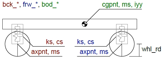
In double roller 3DoF, the wheels remain rigid and follow the road in the same way as a rigid body motion model while the car body is free to move in the Z direction and rotate about the Y axis. This provides two more degrees-of-freedom for a total of three, hence double roller 3DoF. Double roller 3DoF is similar to a half-car model where tire deformation is ignored. With the addition of double roller 3DoF motion alongside its 1DoF counterpart, nanoFluidX now offers the flexibility of choosing the appropriate suspension model in water wading and other compatible cases.
It is recommended to use the 1DoF variant where fluid forces on the body are negligible, such as shallow cases, and to use 3DoF only when interaction with fluid becomes important. In cases where small changes in the road path slope between different segments is small, using the 1DoF variant is sufficient. The 3DoF variant is recommended only when the modeled linear spring/damper response results in non-negligible difference in body position and angle when passing between different road segments.
In addition to wheel radius (dr3dof_whl_rd), body center of mass
(dr3dof_bod_cgpnt) and front and rear axis points
(dr3dof_frw_axpnt), that are common between 1DoF and 3DoF
variants, double roller 3DoF requires body mass (dr3dof_bd_m),
moment of inertia about the Y axis (dr3dof_bod_iyy) and spring
(dr3dof_frw_ks) and damper constants
(dr3dof_frw_cs) for front and rear wheels. Front and rear wheel
masses (dr3dof_frw_ms) are optional. The figure below, Figure 1, marks the
required values on the schematic.
Domain
Definition of the computation domain is important. The domain must extend far enough upstream and downstream of the vehicle to capture the bow wave formed, along with the wake trailing the vehicle. The default values for domain size (thunderbolt icon) consider that vehicle velocity stays below 20 km/h.
Probes and Extractors
Alongside the conventional probes that are used to extract accurate post-processing information at the particular location, it is recommended that you use the extractors in water management simulations. For more information, refer to Probes and Extractors in the Command Reference guide.
Export
Prior to the export of the solver input files, it is recommended to perform a Data Check to avoid possible inconsistencies and errors.