ACU-T: 7203 Thermal Topology Optimization with HeatSink, Utilizing the acu2Topo Utility Script
Tutorial Level: Advanced
Prerequisites
In this tutorial, you will learn how to set up a heat sink flow problem using SimLab, and then transform the flow input file into a thermal topology optimization input file, using the acu2Topo utility script, to incorporate specific objectives and constraints.
Prior to starting this tutorial, you should have already run through the introductory tutorial, ACU-T: 1000 UI Introduction, and have a basic understanding of SimLab, AcuSolve, and EDEM. To run this simulation, you will need access to a licensed version of SimLab, AcuSolve, and EDEM.
Before you begin, copy the file(s) used in this tutorial to your working directory.
Problem Description
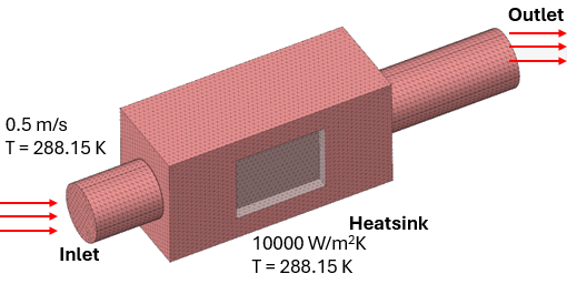
Import the CAD File
- Start SimLab.
- Click .
- Browse to the directory where you saved the model file.
- Select the file HeatSinkCADmodel.slb and then click Open.
Generate the Surface Mesh
-
From the Mesh ribbon, click the Surface Mesh tool.
Figure 2. 
- Select the Element Type as Tri3.
- Enter the Average element size as 2 mm.
- Select the entire model from the modeling window.
-
Click OK.
Figure 3. 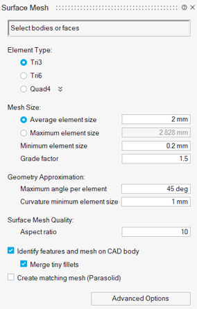
Generate the Interfaces
-
From the Geometry ribbon, click the Connect tool.
Figure 4. 
-
Select Planar faces and
Mesh.
Figure 5. 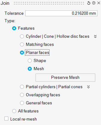
-
Click Show.
Figure 6. . Shows the representation of interfaces 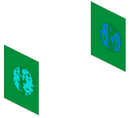
- Click Join.
Generate the Volume Mesh
-
From the Mesh ribbon, click the Tet tool.
Figure 7. 
- For the Element Type, select TET4.
- Enter the Average element size as 1 mm.
-
Click Apply.
Figure 8. 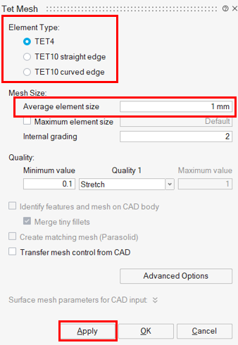
-
Select Replace the mesh in existing model.
Figure 9. 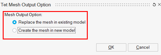
-
Click OK.
Figure 10. 
Define Physics
-
From the Solutions ribbon, click the Flow tool.
Figure 11. 
-
Enter the settings as shown in the Solution dialog.
Figure 12. 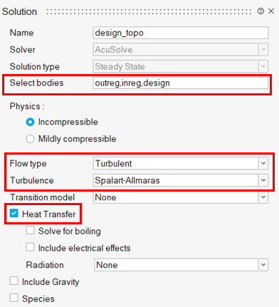
- Click OK.
Define Boundary Conditions
Define Inlet Boundary Condition
-
From the Analysis ribbon, click the Inlet tool.
Figure 13. 
- Select Inlet surface.
-
Enter the settings as shown in the Inlet dialog.
Figure 14. 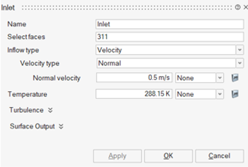
- Click OK.
Define Outlet Boundary Condition
-
From the Analysis ribbon, click the Outlet tool.
Figure 15. 
-
Select the outlet surface, as shown in the figure.
Figure 16. 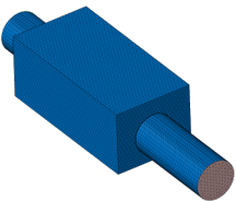
-
Enter the settings as shown in the Outlet dialog.
Figure 17. 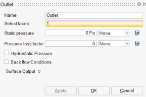
- Click OK.
Define Wall Boundary Condition to Heatsink
-
From the Analysis ribbon, click the Wall tool.
Figure 18. 
-
Click the surfaces of the heatsink, as shown below.
Figure 19. 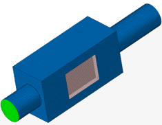
-
Enter the settings as shown in the Wall dialog.
Figure 20. 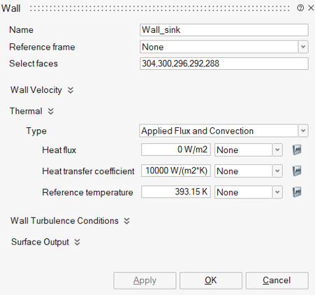
- Click OK.
Define Wall Boundary Condition to Outer Wall
-
From the Analysis ribbon, click the Wall tool.
Figure 21.
-
Click all of the six surfaces of the outer box, as shown in figure below.
Figure 22. 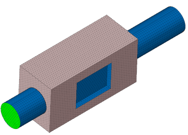
-
Enter the settings as shown in the Wall dialog.
Figure 23. 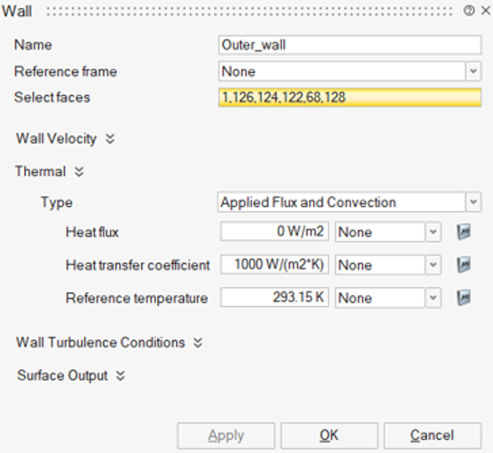
- Click OK.
Define Solver Settings
- From the Solution Browser, click Settings.
-
Enter Maximum no. of time steps as 100, Convergence
tolerance as 0.0001 and Number of Krylov vectors as
40.
Figure 24. 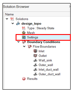
Figure 25. 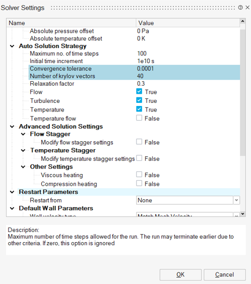
- Click OK.
Define Result Request Settings
- From the Solution Browser, right-click Settings and select Result Request.
-
Enter Output frequency and No. of saved states as 1000
and 2000, respectively.
Figure 26.
Figure 27. 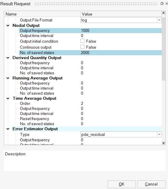
- Click OK.
Export Flow Solver Input Deck
- From the Solution Browser, right-click design_topo and select Export Solver Input File.
- Enter the input file name as HeatSink.
Run AcuSolve
- From the Results ribbon, click the drop-down arrow next to Results and select Command Prompt.
-
Specify the problem directory and execute the following command:
python3 acu2Topo.py -i HeatSink.inp -o heatsink_tut_therm.inp -f -r 0.005 -t -obj "maximize temperature" -con "mechanical energy less than" "design fraction greater than" -b 3.5e-5 0.2
Figure 28. 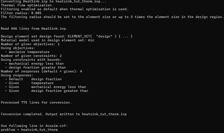
The new input file heatsink_tut_therm.inp is created.
- Enter the problem name as heatsink_tut_therm and add display_design_topology = TRUE in the Acusim.cnf file.
- Change the conductivity of Air_design to 100 in the input file.
-
Execute the simulation run with the following command:
acuRun –np 8 –nt 1The simulation run completes in about 9 hours.
Post-Process the Results with SimLab
- Click .
- Select the heatsink_tut_therm.1.Log file and click Open.
-
From the Results ribbon, click the Iso Surface
tool.
Figure 29. 
-
For Show Contour select Below and then click
Apply.
Figure 30. 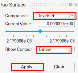
Figure 31. 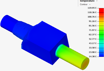
-
Click
 to enable
the Cutting Plane option.
to enable
the Cutting Plane option.
-
Click
 to enable
the Flip Cutting Plane option and close the Cutting Plane option.
to enable
the Flip Cutting Plane option and close the Cutting Plane option.
- In the modeling window, right-click and select Redisplay Model.
-
Click to enable
the Cutting Plane option and hide the two non-design volumes.
Figure 32. 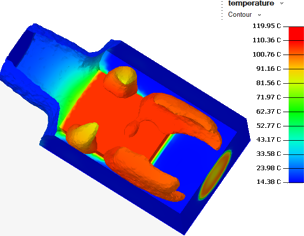
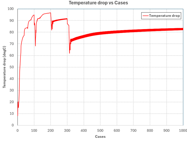
Post-Process the Results with acuGetRsp
-
Open the command prompt and execute the following command:
acuGetRsp>Rsp.txtThis generates the file name as Rsp.txt in the working directory.
The second column in Rsp.txt corresponds to temperature drop.
-
To visualize the temperature plot, import Rsp.txt in
Microsoft Excel.
Results are plotted, as shown below.
Figure 33.