ACU-T: 5100 Modeling of a Fan Component Using the Fan Component - Coefficient Method

Prerequisites

This simulation provides instructions for modeling a fan using the classic fan component. Prior to starting this tutorial, you should have already run through the introductory tutorial, ACU-T: 1000 UI Introduction, and have a basic understanding of HyperMesh CFD and AcuSolve. To run this simulation, you will need access to a licensed version of HyperMesh CFD and AcuSolve.

Before you begin, copy the file(s) used in this tutorial to your working directory.

Note: This tutorial does not cover the steps related to geometry cleanup and mesh settings.

Problem Description

The problem to be solved in this tutorial is shown schematically in the figure below. It consists of an interior fan which rotates at a speed of 377 rad/sec (~3600 RPM) and has a thickness of 0.06 m and a tip radius of 0.11 m. The volumetric flow rate at the inlet is 0.322675 m³/sec (~1161.63 m³/hr). The problem is simulated as a steady state run and the pressure rise across the fan region is computed.

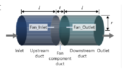
Figure 1 shows a simple axial fan component problem where the fan is an interior fan with thickness “t” and tip radius “r”. In this simulation, flow is passed from the pipe inlet. It enters the fan in an axial direction and exits at the outlet causing pressure rise. This fan pressure rise can be simulated for a given volume flow rate at the inlet surface which will be assigned as the inflow boundary condition. The middle portion of the pipe is the Fan Component which has both Fan_Inlet and Fan_Outlet.

The Fan Component directly computes the body force term to yield the pressure rise within the volume of interest. The body force is applied directly to the volume and not the surface. In order to yield the required pressure rise based on fan performance curve that the you have input, you need to evaluate the volume flow rate correctly at the inlet surface of the domain.

A fan component is modeled by adding the body force to the momentum equations, which increases the pressure across the component by:

Δ P_{a x i a l} = \frac{1}{2} α_{a x i a l} ρ u_{t i p}^{2} + \frac{1}{2} ρ {\bar{u}}^{2}

Where:

$α_{a x i a l}$ - axial coefficient of the fan component
$u_{t i p}^{}$ - tip velocity (m/sec) = $ω r_{t i p}$
$ω$ - fan angular rotational speed (rad/sec)
$r_{t i p}$ - fan tip radius (m)
$\bar{u}$ - mass averaged velocity (m/sec) through inlet

The fan pressure rise is determined by the fan performance (P-Q) curve which is mainly dependent on the volume flow rate and fan speed for the required fan pressure rise (∆P). Since piecewise_bilinear curve fit values used in the classic FAN_COMPONENT approach are functions of the normalized flow rate and axial coefficient, you need to convert them from the fan performance curve.

Normalized flow rate $(Q^{l}) = \frac{Q}{A u_{t i p}}$

Where:

Q - flow rate
A - area

Axial coefficient $(α_{a x i a l}) = \frac{2 Δ P - ρ {\bar{u}}^{2}}{ρ u_{t i p}^{2}}$

For example, evaluate the axial coefficients and normalized flow rate from the fan performance data. The following tables are inputs for the calculations.

Table 1. Fan characteristics
Fluid Density	1.225 kg/m³
Tip Radius ( $r_{t i p}$ - fan tip radius (m))	0.11m
Rotational Speed ( $ω$ )	3600 RPM = 376.99 rad/sec
Inlet Area, A_i	0.03801 m²
Tip Velocity ( $u_{t i p}^{}$ )	41.47 m/sec

Table 2. Fan performance parameters
S.No	Volume flow rate (Q), m³/hr	Pressure rise (dP), Pa
1	525.35	494.91
2	890.21	474.63
3	1161.63	424.90
4	1272.76	389.11
5	1356.57	350.42
6	1431.84	308.18
7	1494.69	268.35
8	1551.39	230.89

You can calculate the normalized flow rate and axial coefficient for first two volume flow rates (Q) from Table 2. The same procedure is followed for the other volume flow rates.

For Q = 525.35 m³/hr:

$\begin{array}{l} Q^{1} = \frac{Q}{A u_{t i p}} = 0.0926 \\ α_{a x i a l} = \frac{2 Δ P - ρ {\bar{u}}^{2}}{ρ u_{t i p}^{2}} = 0.4613 \end{array}$
For Q = 890.21 m³/hr:

$\begin{array}{l} Q^{1} = \frac{Q}{A u_{t i p}} = 0.1569 \\ α_{a x i a l} = \frac{2 Δ P - ρ {\bar{u}}^{2}}{ρ u_{t i p}^{2}} = 0.426 \end{array}$

In this manner we calculate Q^l and α_axialfor the remaining volume flow rates, shown in the following table.

Table 3. Normalized flow rates and axial coefficients
S.No	Normalized flow rate (Q^l)	Axial Coefficients (α_axial)
1	0.0926	0.4613
2	0.1569	0.426
3	0.2047	0.3615
4	0.2243	0.3191
5	0.239	0.2755
6	0.2523	0.229
7	0.2634	0.1854
8	0.2734	0.1445

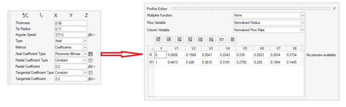
The same information is entered as input for the FAN_COMPONENT parameter as shown below in Figure 2.

The first column (0,1) is the normalized radius and the first row (0.0926,…,0.2734) defines the normalized flow rate. The second row data (0.4613,…,0.1445) are for the axial coefficient.

Start HyperMesh CFD and Open the HyperMesh Database

Start HyperMesh CFD from the Windows Start menu by clicking Start > Altair <version> > HyperMesh CFD.
From the Home tools, Files tool group, click the Open Model tool.

Figure 3.

The Open File dialog opens.
Browse to the directory where you saved the model file. Select the HyperMesh file ACU-T5100_CoefficientFanComponent.hm and click Open.
Click File > Save As.
Create a new directory named Axial_Fan and navigate into this directory.
This will be the working directory and all the files related to the simulation will be stored in this location.
Enter Axial_Fan as the file name for the database, or choose any name of your preference.
Click Save to create the database.

Validate the Geometry

The Validate tool scans through the entire model, performs checks on the surfaces and solids, and flags any defects in the geometry, such as free edges, closed shells, intersections, duplicates, and slivers.

To focus on the physics part of the simulation, this tutorial input file contains geometry which has already been validated. Observe that a blue check mark appears on the top-left corner of the Validate icon on the Geometry ribbon. This indicates that the geometry is valid, and you can go to the flow set up.

Set Up Flow

Set the General Simulation Parameters

From the Flow ribbon, click the Physics tool.

Figure 5.

The Setup dialog opens.
Under the Physics models setting:
1. Verify that Time marching is set to Steady.
2. Select Spalart-Allmaras as the Turbulence model.
Figure 6.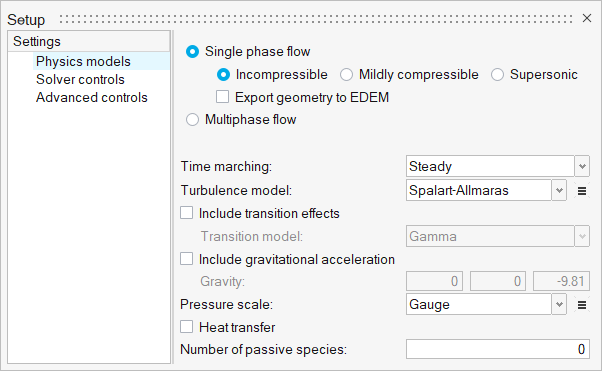
Click the Solver controls setting and verify that the parameters are set as shown in the figure below.

Figure 7.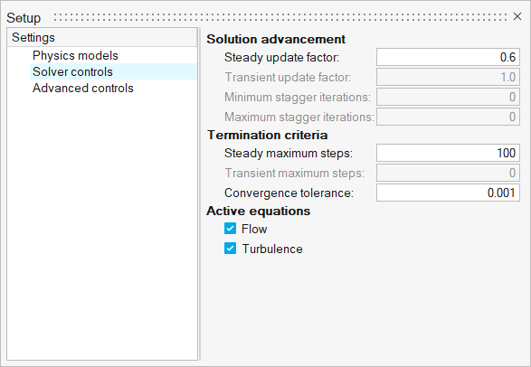
Close the dialog and save the model.

Assign Material Properties

From the Flow ribbon, click the Material tool.

Figure 8.
Verify that the Air material has been assigned to all three volumes.
Click on the guide bar to exit the tool.

Define the Fan Component

From the Flow ribbon, click the arrow next to the Domain tool set, then select Fan Component.

Figure 9.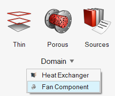
Select the middle solid as the fan component volume.

Figure 10.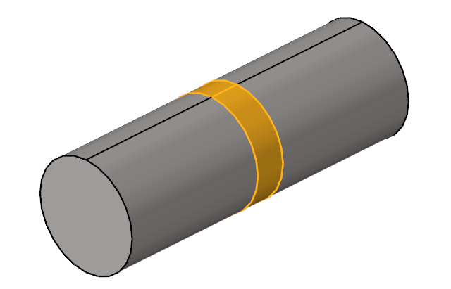
On the guide bar, click Surfaces then select the face shown below as the inlet of the fan component.

Figure 11.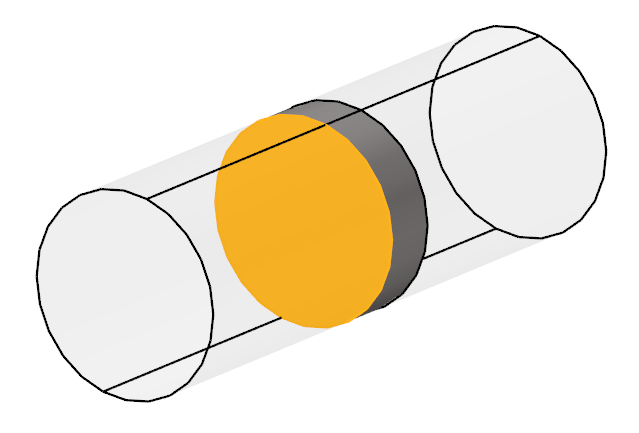
From the View Controls toolbar, change the geometry visualization mode from Shaded Geometry to Transparent Geometry.

This allows you to view the axis direction vector in the next step.
Figure 12.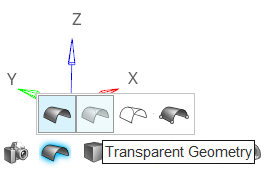
On the guide bar, click Axis.
In the modeling window, you can see that the axis points in the -X direction.
Click in the microdialog to flip the axis vector to the +X direction.

Figure 13.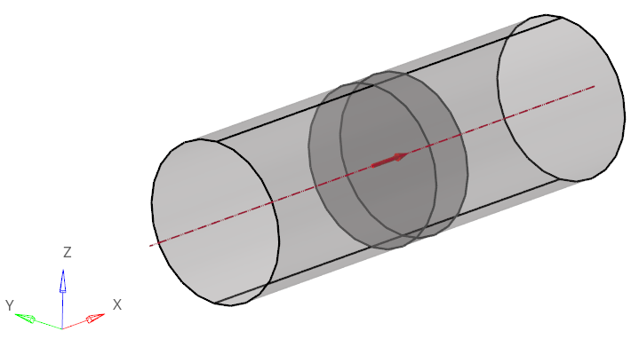
Enter 0.06 for Thickness (m).
Set the Type to Axial and set the Method to Coefficients.
Enter 0.11 for Tip Radius (m) and 377 for Angular Speed (rad/sec).
Set the Axial Coefficient Type to Piecewise Bilinear.

Figure 14.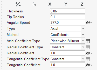
Click beside Piecewise Bilinear to open the Profile Editor.
Click , browse to the location where you saved FanAxialCoefficients.csv, and open it.

Figure 15.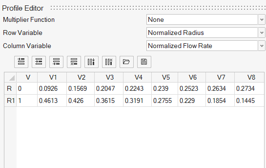

Note: Both Normalized flow rate and Axial Coefficients have non-dimensionless units
Ensure that Row Variable is set to Normalized Radius and Column Variable to Normalized Flow Rate.
Close the Profile Editor.
Change the Radial Coefficient and Tangential Coefficient values from 1.0 to 0.0.

Figure 16.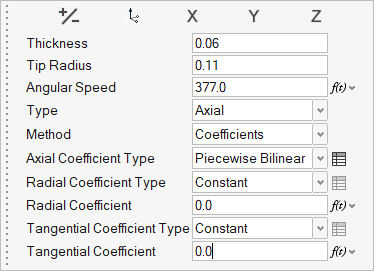

Note: Make sure that both Radial and Tangential coefficient values are set to 0 since the fluid enters only in the axial direction.
On the guide bar, click to execute the command and exit the tool.
Save the model.

Define Flow Boundary Conditions

From the Flow ribbon, Profiled tool group, click the Volumetric Flow Rate tool.

Figure 17.
Click the inlet face highlighted in the figure below.

Figure 18.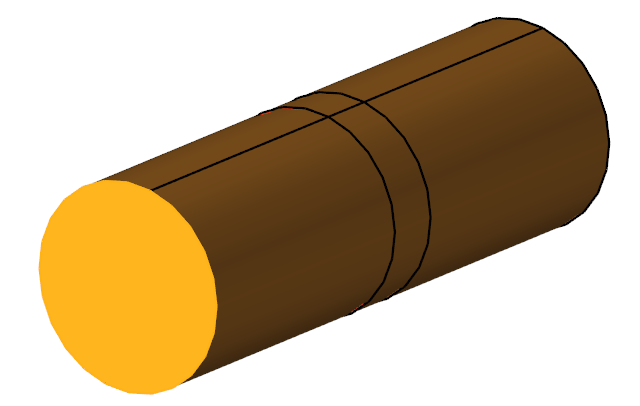
In the microdialog, enter 0.322675 for the volumetric flow rate (m³/sec).

Figure 19.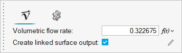
On the guide bar, click to execute the command and exit the tool.
Click the Outlet tool.

Figure 20.
Select the face highlighted in the figure below and then click on the guide bar.

Figure 21.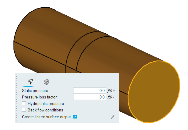

Generate the Mesh

To focus on the solver setup, the mesh settings are predefined in the input file given to you.

From the Mesh ribbon, click the Volume tool.

Figure 22.
In the Meshing Operations dialog, set the Average element size to 0.01 and the Mesh growth rate to 1.1 (if not set already).

Figure 23.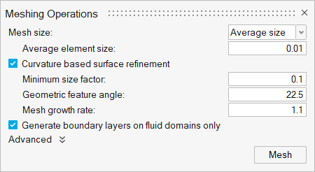
Click Mesh.
The Run Status dialog opens. Once the run is complete, the status is updated and you can close the dialog.
Tip: Right-click on the mesh job and select View log file to view a summary of the meshing process.
Save the model.

Define Surface Monitors and Run AcuSolve

Set the entity selector to Solids.

Figure 24.
Select the fan component duct marked below to isolate it from front and aft ducts.

Figure 25.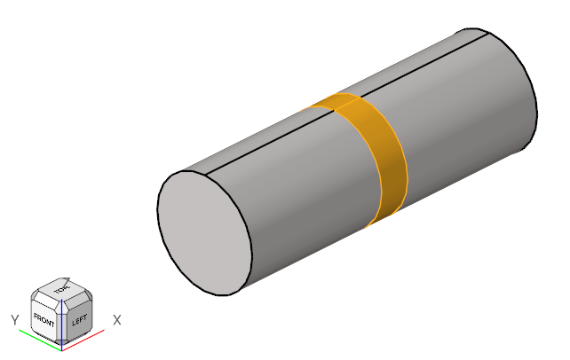
Right-click and select Isolate form the context menu or press I.
The solid for the fan component should be displayed in the modeling window.
Figure 26.
Form the Solution ribbon, click the Surfaces tool.

Figure 27.
Select the front face of the fan and verify that the arrow is heading toward the fan component, as shown in figure below

Figure 28.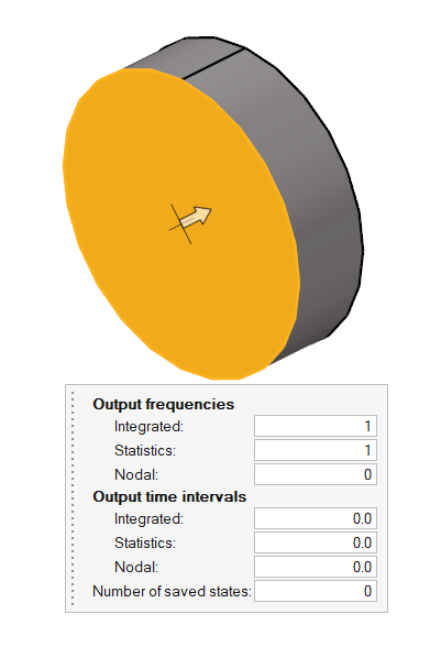
On the guide bar, click to execute the command and remain in the tool.
In the legend, rename surface_output to FAN_inlet.
Rotate the fan component and select the rear face.

Figure 29.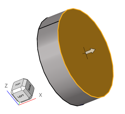
Click , rename surface_output to FAN_outlet in the legend, then click to exit the tool.
From the Solution ribbon, click the Run tool.

Figure 30.

The Launch AcuSolve dialog opens.
Set the Parallel processing option to Intel MPI.
Optional: Set the number of processors to 4 or 8 based on availability.
Leave the remaining options as default and click Run to launch AcuSolve.

Figure 31.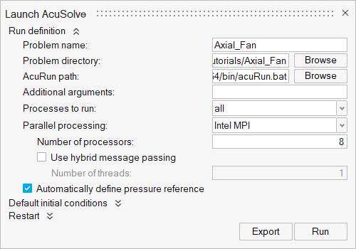

Post-Process with the Plot Tool

From the Solution ribbon, click the Plot tool.

Figure 32.

Figure 33.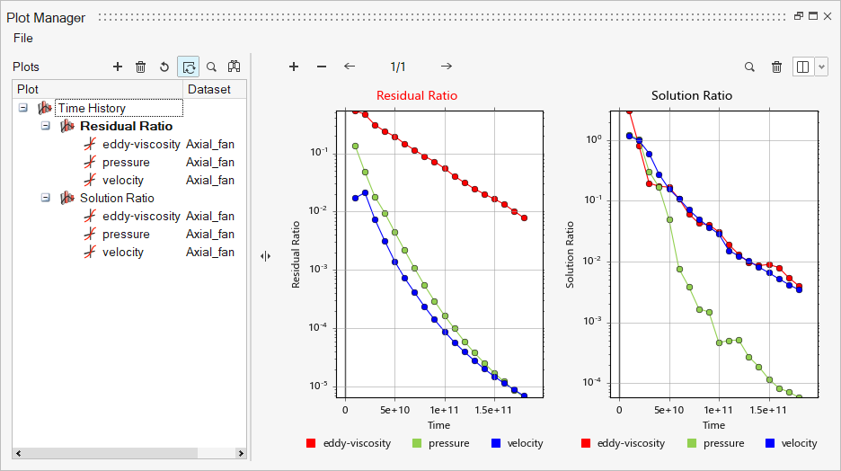
Click to create a new plot.
In the Data Tree, expand Integrated Surface Output > Pressure then select pressure.
Under Parts, select Fan_inlet and Fan_oultet to display pressure at the inlet and outlet.

Figure 34.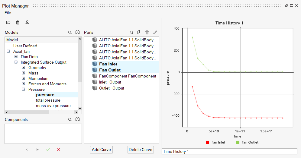
Right-click User Defined under the Model panel to create a user defined function.
In the Data Tree, expand Integrated Surface Output > Pressure then select pressure.
In the Name field, enter dP.
In the Value field, type value=.
Under Parts, choose FAN outlet then click to insert the field as part of the value, as shown below.

Figure 35.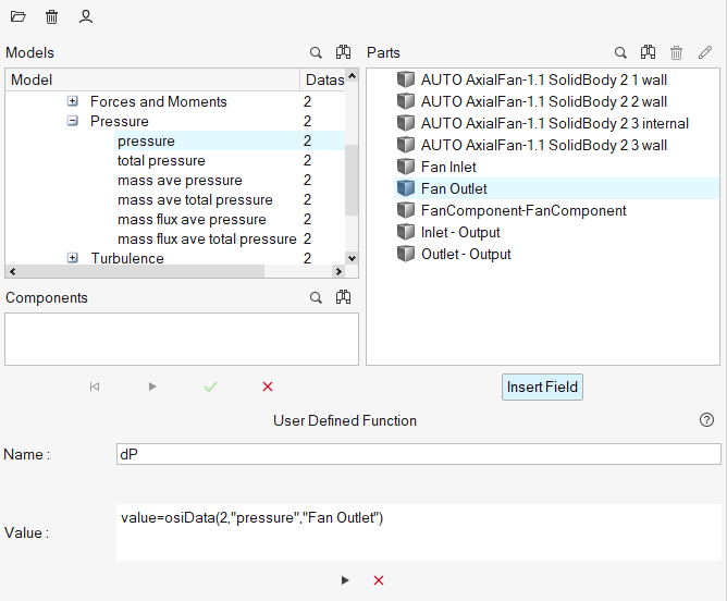
Type - at the end of the user defined function value.
Under Parts, choose FAN inlet then click to insert the field as part of the value.
Click to add the user defined function.

Figure 36.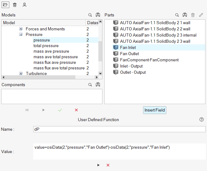
Click the x axis to switch to Time Steps.

Figure 37.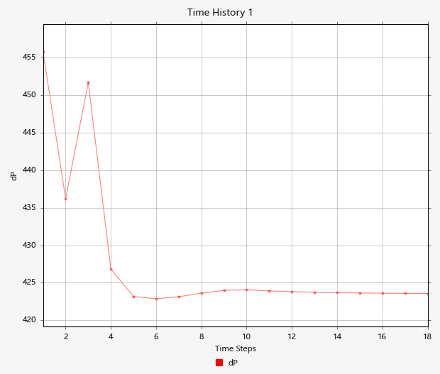

From the above figure, the pressure got stabilized at around the 6^th iteration and remains constant with pressure difference between the FAN_inlet and FAN_outlet of 423.97 Pa for a given volume flow rate 0.322675 m³/sec, which is very near compared to the reference pressure increase of 424.9 Pa.

Summary

In this tutorial, you successfully learned how to set up and solve a simulation involving a coefficient fan component using HyperMesh CFD. You imported the geometry and then defined the simulation parameters, coefficient fan component, and flow boundary conditions. Once the solution was computed, you used the HM-CFD Plot tool to plot the pressure at fan inlet and fan outlet.