
ACU-T: 5001 Blower - Transient (Sliding Mesh)
Tutorial Level: Beginner
Prerequisites
This tutorial provides the instructions for setting up, solving, and viewing results for a transient simulation of a centrifugal air blower utilizing the sliding mesh approach. In order to run this tutorial, you should have already run through ACU-T: 5000 Blower - Steady (Rotating Frame) and kept the solution in your working directory. It is assumed that you have some familiarity with HyperMesh CFD and AcuSolve. To run this simulation, you will need access to a licensed version of HyperMesh CFD and AcuSolve.
Since the HyperMesh CFD database (.hm file) uses the ACU-T:5000 Blower-Steady model, this tutorial skips the geometry clean-up and inlet boundary conditions as well as the mesh settings.
Problem Description
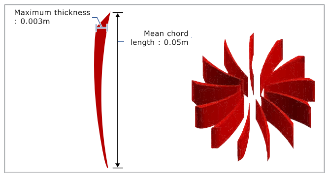
The problem to be addressed in this tutorial is shown schematically in Figure 1 and Figure 2. It consists of a centrifugal blower with forward curved blades. The fluid through the inlet plane enters the hub of the blade wheel, radially accelerates due to centrifugal force as it flows over the blades, and then exits the blower housing through the outlet plane.

To capture the dynamic motion of the impeller blades, the simulation must be transient. The time step size is determined by:
where ω is the blower rotational speed. It should be noted that a time step size sensitivity study should always be performed to establish appropriate time step size when analyzing a new application.
The CFD analysis of this problem offers detailed information about the flow through a centrifugal blower. To investigate this behavior, it is necessary to select an appropriate set of boundary conditions to use. There are two different methods that are commonly used. One approach is to specify the mass flow rate at the inlet of the blower and allow AcuSolve to compute the pressure drop, that is, flow forces simulation. Another option is to specify the stagnation pressure at the inlet and allow AcuSolve to compute the flow rate that results from this specified pressure change between the inlet and outlet. The boundary conditions used in this example are the latter. That is, the inlet is taken as stagnation pressure rather than mass flow rate so that AcuSolve calculates mass flow rates and pressure rise based on impeller rotation.
The fluid in this problem is air, which has a density of 1.225 kg/m3 and a viscosity of 1.781 X 10⁻⁵ kg/m-s.
Start HyperMesh CFD and Open the HyperMesh Database
- Start HyperMesh CFD from the Windows Start menu by clicking .
-
From the Home tools, Files tool group, click the Open Model tool.
Figure 3. 
The Open File dialog opens. - Browse to the directory where you saved the model file. Select the HyperMesh file ACU-T5001_BlowerTransient.hm and click Open.
- Click .
-
Create a new directory named BlowerTransient and navigate into this directory.
This will be the working directory and all the files related to the simulation will be stored in this location.
- Enter BlowerTransient_solved as the file name for the database, or choose any name of your preference.
- Click Save to create the database.
Set Up Flow
Set Up the Simulation Parameters and Solver Settings
-
From the Flow ribbon, click the Physics tool.
Figure 4. 
The Setup dialog opens. -
Under the Physics models settings:
- Set Time marching to Transient.
- Set the Time step size to 0.0005 and the Final time to 0.05.
Figure 5. 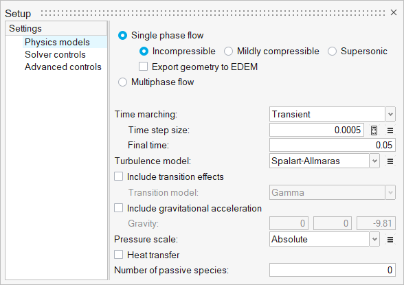
- Click Solver controls.
-
Set the Minimum stagger iterations and Maximum stagger iterations to
2 and 6, respectively.
Figure 6. 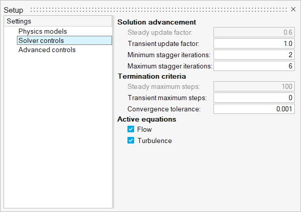
- Close the dialog and save the model.
Define Flow Boundary Conditions
-
From the Flow ribbon, Pressure
tool group, click the Stagnation Pressure tool.
Figure 7. 
-
Click the face of the inlet.
Figure 8. 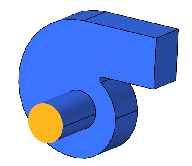
- In the microdialog, click the Turbulence tab.
- Set the Turbulence input type to Auto.
-
Set the Turbulence flow type to Internal.
Figure 9. 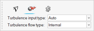
-
Rename the inlet.
- From the legend on the left side of the modeling window, double-click Stagnation pressure.
- Type Inlet and press Enter.
-
On the guide bar, click
 to execute
the command and exit the tool.
to execute
the command and exit the tool.
-
Click the Outlet tool.
Figure 10. 
-
Click the face of the outlet.
Figure 11. 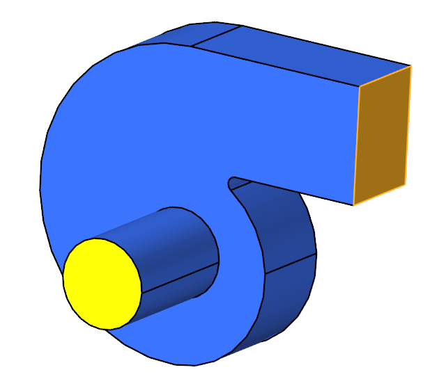
-
In the microdialog, make sure both Static pressure and Pressure loss
factor are 0.
Figure 12. 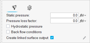
-
On the guide bar, click
to execute
the command and exit the tool.
Set Up Mesh Motion
Define the Mesh Motion Type
-
From the Motion ribbon, click the Settings tool.
Figure 13.
The Setup dialog opens. - Change the Mesh motion type to Specified.
- Click the Solver controls setting and make sure the Mesh deformation checkbox is checked.
Define the Rotating Mesh Motion
-
Hide the housing solid.
- Set the entity selector to Solids.
- Select the centrifugal housing.
- Right-click and select Hide or press H on your keyboard.
Figure 14. 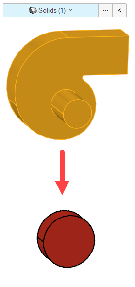
-
Click the Rotation tool.
Figure 15. 
- Select the solid in the modeling window.
- On the guide bar, click Axis.
-
Define the axis of rotation.
-
Use the Surf Center snap point to place the axis in the middle of the
centrifugal blower.
Figure 16. 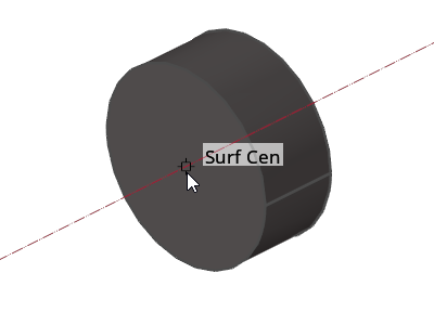
-
Click
 to change the rotational direction.
Figure 17. 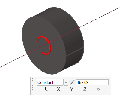
-
Use the Surf Center snap point to place the axis in the middle of the
centrifugal blower.
-
On the guide bar, click
to execute
the command and exit the tool.
- Right-click in the modeling window and select Show All or press A on your keyboard to return to the full model view.
Define Nodal Output Frequency
-
From the Solution ribbon, click the Field tool.
Figure 18. 
The Field Output dialog opens. - Check the Write initial conditions checkbox.
- Check the Write results at time step interval checkbox.
-
Set the Time step interval to 1.
Figure 19. 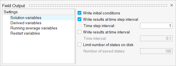
Run AcuSolve
-
From the Solution ribbon, click the Run tool.
Figure 20. 
- Set the Parallel processing option to Intel MPI.
- Optional: Set the number of processors to 4 or 8 based on availability.
- Deactivate the Automatically define pressure reference option.
-
Leave the remaining options as default and click
Run to launch AcuSolve.
Figure 21. 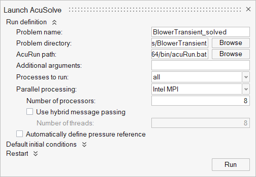
Tip: While AcuSolve is running, right-click the AcuSolve job in the Run Status dialog and select View Log File to monitor the solution process.
Post-Process the Results with HM-CFD Post
- Navigate to the Post ribbon.
- From the menu bar, click .
-
Select the AcuSolve
.log file in your problem
directory to load the results for post-processing.
The solid and all the surfaces are loaded in the Post Browser.
-
Click the Slice Planes tool.
Figure 22. 
- Select the x-y plane in the modeling window.
-
In the microdialog, click
 and move the plane along its normal direction a distance of
-0.07.
and move the plane along its normal direction a distance of
-0.07.
Figure 23. 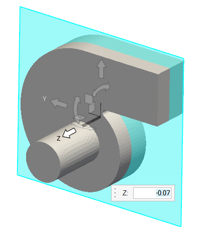
- Press Esc to exit the Move tool context.
-
In the slice plane microdialog, click
 to
create the slice plane.
to
create the slice plane.
- In the display properties microdialog, toggle the Legend radio button and set the bounds to -120 and 43.
-
Click
 and set the Colormap Name to Rainbow
Uniform.
and set the Colormap Name to Rainbow
Uniform.
Figure 24. 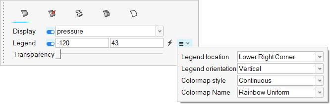
-
On the guide bar, click
to execute
the command and exit the tool.
- In the Post Browser, hide all the Parts and Flow Boundaries.
-
Click the play button on the Animation toolbar.
Figure 25. 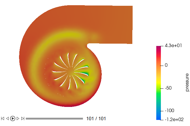
- Click to save the pressure contour animation.
Summary
In this tutorial, you worked through a basic workflow to set up a transient simulation with a sliding mesh in a centrifugal blower. You started by importing the mesh; once the case was set up, you generated a solution using AcuSolve. Then, you computed the blower momentum using the Plot tool and created a contour plot for pressure on a cut plane using HyperMesh CFD post.