Isovalues: compute and display
Computing and displaying isovalues
To compute isovalues, the user has to:
| Step | Action | |
|---|---|---|
| 1 | In the Post processing menu, select Isovalues on conductors or Isovalues on 2D grids and then click on one of the spatial quantities available | |
| 2 |
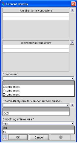
In the dialog box that appears:
|
|
| → | The isovalues are calculated and displayed on the support selected in the graphic window. | |
Note: * If the spatial quantity chosen is a scalar quantity (for instance the Joule
losses density) the "Component" and "Coordinate
system for component computation" slots are not displayed as the
modulus of the spatial quantity is automatically considered.
Isovalues graphic window
The isovalues are displayed in the graphic window whose appearance and look change as shown in the figure below.
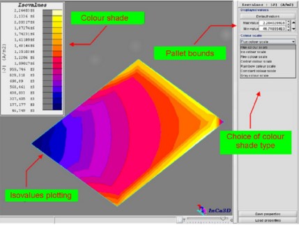
It contains the following zones:
- the isovalues plotting on the supports previously selected by the user
- the color shade which specifies the correspondence between the color shade and the spatial values displayed on the supports; this pallet can be resized and/or moved on the isovalues plotting by means of the mouse in order to distinguish more easily the value of the spatial quantity at each point of the support
- the pallet bounds, i.e. the limits of the color shade; these values can be changed by the user
- the menu for the choice of color shade type to use for the plotting of the isovalues on the supports