Plotting a 2D spatial curve
Definition
A 2D spatial curve represents for a given frequency the evolution of a local (scalar) physical quantity on a support of path type.
The choice of the frequency is done by selecting a step from the solving scenario .
Physical quantity
The physical quantities that can be displayed with 2D spatial curves are:
- current density
- Joule losses density
- magnetic flux density
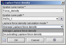
- Laplace force density: average component as well as 2ω pulsating component
As regards the current density, the magnetic flux density and the pulsating component of the Laplace force, the curves representing the magnitude, the phase, the real part and the imaginary part of each component (X, Y and Z) are created and displayed; representing altogether twelve curves.
For the average component of the Laplace force the curves representing the values taken by the three components (X, Y and) are created and displayed.
Creating and displaying 2D spatial curves
To create and display a new 2D spatial curve, the user has to:
| Step | Action | Result |
|---|---|---|
| 1 |
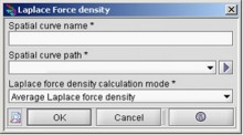
Open one of the 2D spatial curve dialog boxes:
Current density or Losses density or Magnetic flux density or Laplace force density |
|
| 2 |
In the dialog box that appears:
|
|
| → | The 2D curves are displayed in a new specific sheet with the name of the physical quantity considered. | |