Curve Fitting

Each prepared curve is displayed in the Curve Fitting list. Select the desired curve for fitting.

1. Choose the most appropriate approach and select the range of the x-axis (default value is 100%) and then click Curve Fit.
   Each fit is listed in the Extrapolation field. The corresponding curve is plotted in the graph for validation. The Spline option starts a special tool for creating splines.

   
   
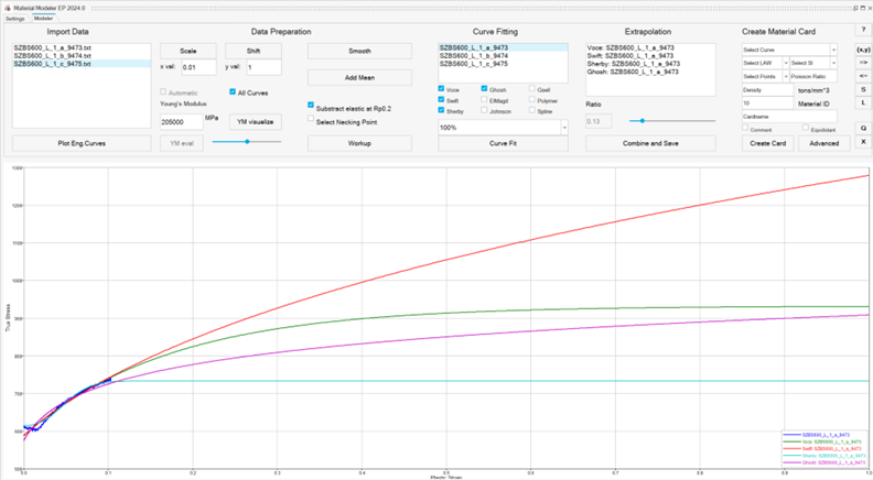
   Figure 1. Corresponding Curve plot for Validation

2. Select a curve in the Extrapolation field. The curve will zoom in and plot the derivative. This indicates:

3. Select one more fitting curve by holding down the control key and clicking with the left mouse button. Adjust the ratio between both curves using the slider. If you are satisfied with the result, click Combine and Save.

   
   
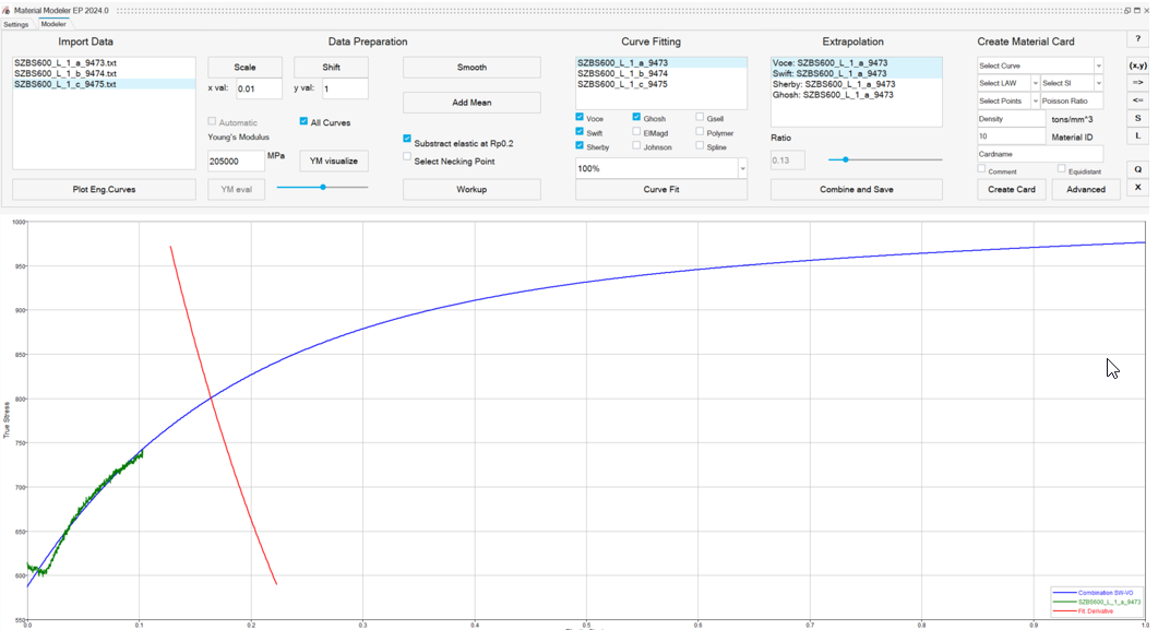
   Figure 2. Combine and Save the Curves

4. Spline is special tool for creating splines. Select the Spline check box, a new window displays with the actual selected curve. You can start redrawing a smoothed curve on the existing curve and re-interpret the hardening curve by adding new points on the existing curve.
5. Interpret and manually add six points, the spline appears, and the line is drawn. Select further points to extrapolate to 100% (or beyond). The dashed curve shows the 1st derivative of the spline.

The crossing points indicate the stability points:

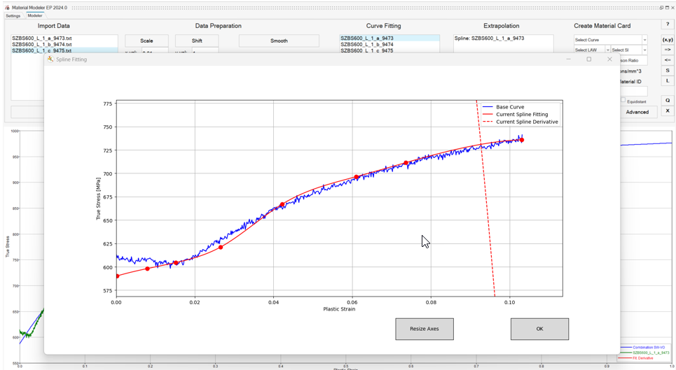
Figure 3. Spline Extrapolation

6. Optional: You can further modify the curve by adding new control points or moving existing ones. The derivative curve is updated to reflect the changes in terms of the numerical material behavior.
   Hardening curves created by spline fitting cannot be used in combination with curves created by extrapolation methods.