Example 1: Monostatic RCS of a Sphere and a Box
In this example, the Monostatic RCS of a box and a sphere is calculated.
Step 1
Start newFASANT.
Step 2
Select File and click on New.
Step 3
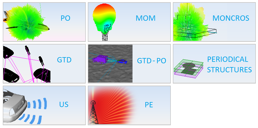
Select GTD-PO.
Step 4
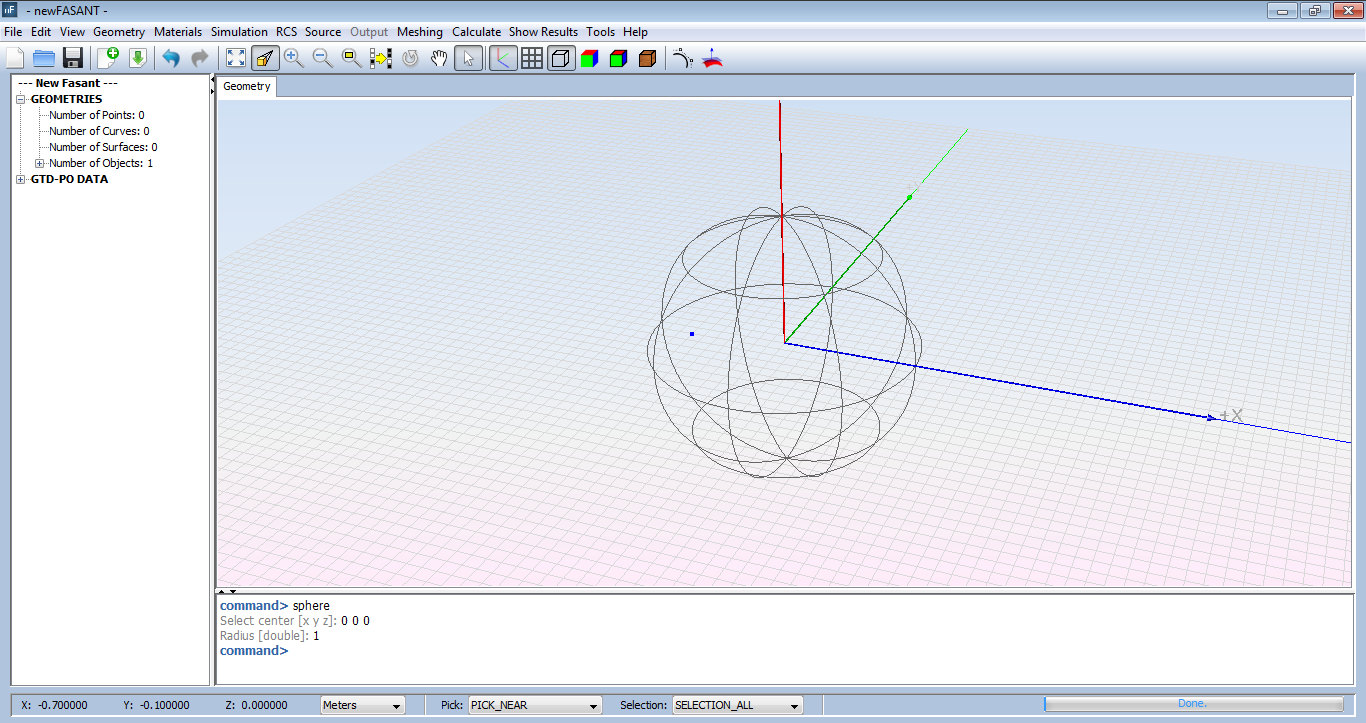
Click on Geometry→Solid→Sphere, which requires the center and the radius, as shown in the next Figure.
In this example the user enters the following values into the command line:
- Center: 0 0 0
- Radius: 1.0
Step 5
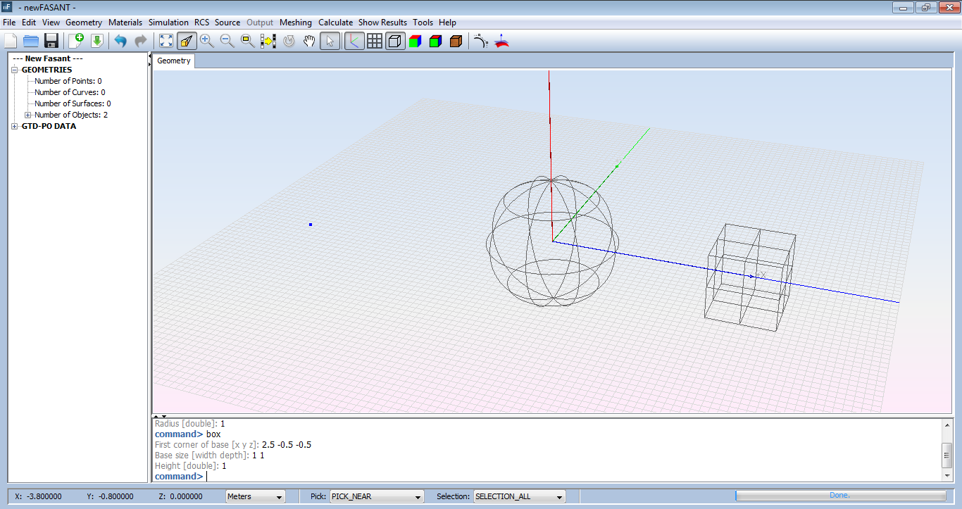
Click on Geometry → Solid → Box, which requires the first corner of the base, width, depth, and height as shown in the next Figure.
In this example the user enters the following values into the command line:
- First corner base: 2.5 -0.5 -0.5
- Width: 1.0
- Depth: 1.0
- Height: 1.0
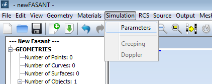
Step 6
Click on Simulation → Parameters.
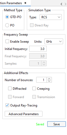
Step 7
On the top left side of the newFASANT window, the user can enter the desired parameters for this simulation, as shown in next Figure.
Select 1 bounce (simple reflection) and a frequency of 3.0 GHz and left-click the Save button.
Step 8
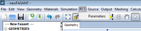
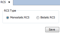
Select RCS → Parameters.
Step 9
This command appears at the top left side of the newFASANT window as shown in the next Figure.
Select Monostatic RCS only.
Step 10
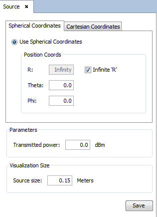
Select Source→ Parameters.
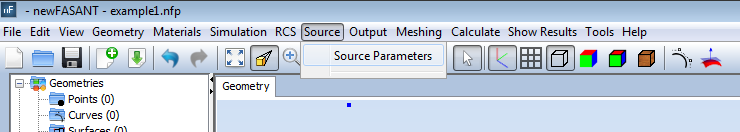
Step 11
Introduce the source position (r, theta, and phi), as shown in the next Figure and left-click on the Save button.
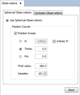
Step 12
In the Output tab, introduce the observation information sweep on theta with 181 samples.
Step 13
Before running the case, select Meshing → Create Mesh.
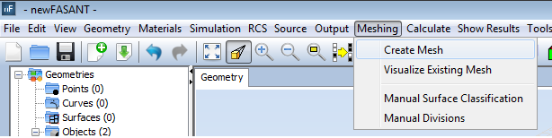
Step 14
Select 1 processor and define the curvature mesh option with a distance error of 0.01 and surface error of 0.08 and left-click on Mesh.
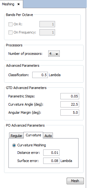
Left-clicking on Mesh launches the meshing engine as shown in the next Figure:
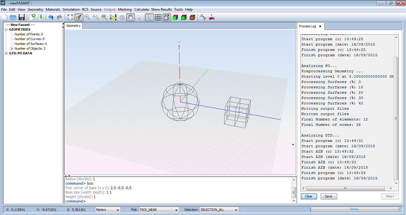
Step 15
To obtain information about the mesh, select Meshing →Visualize Existing Mesh.
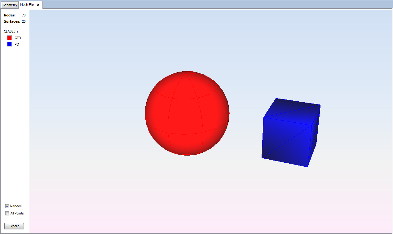
Step 16
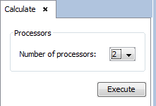
Select Calculate → Execute and select the number of processors available to simulate this case.
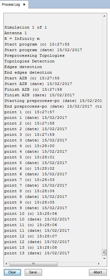
Step 17
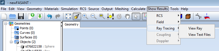
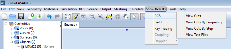
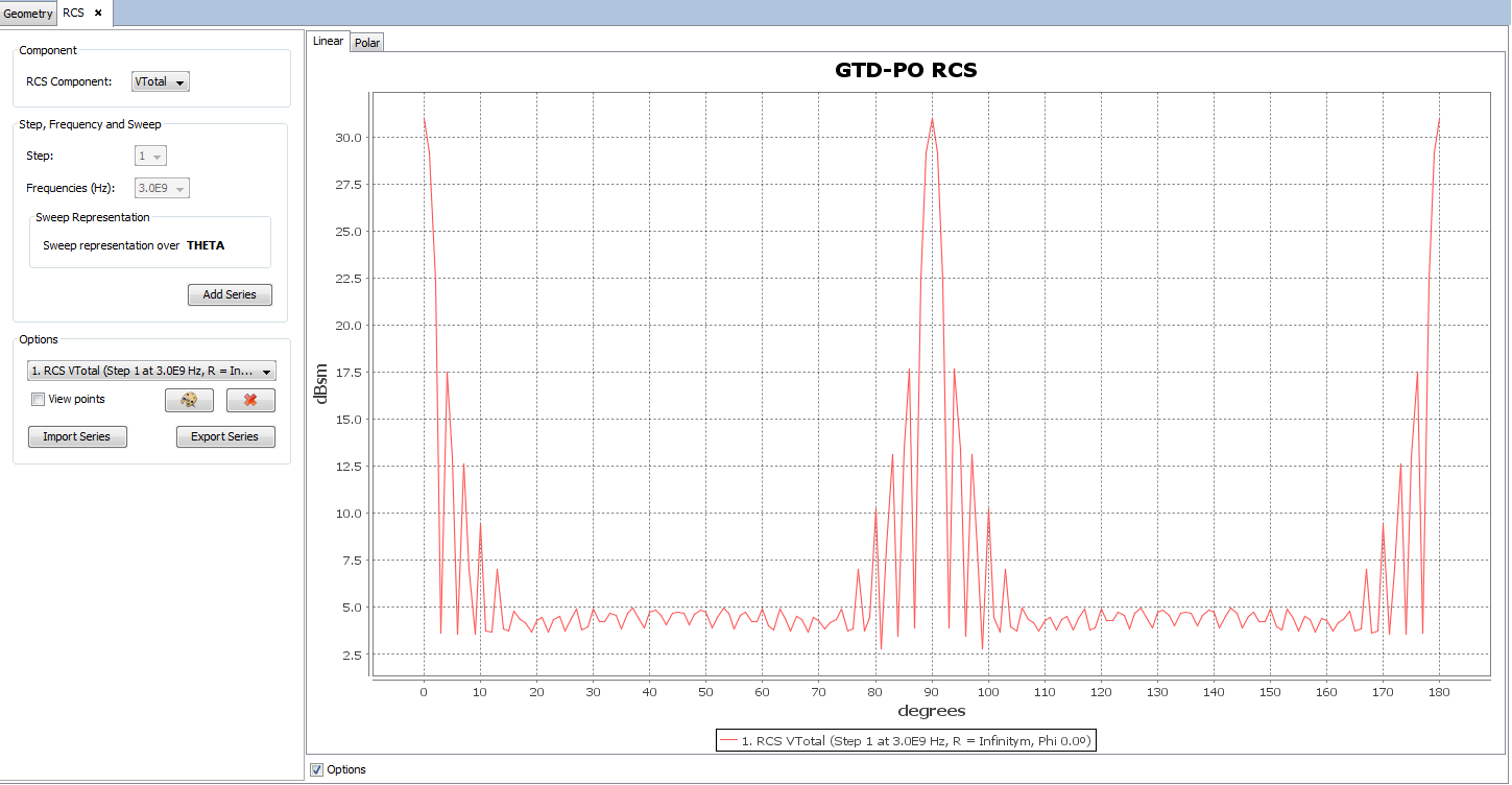
When the simulation finishes we can visualize the simulation results. Click on Show Results →RCS→ View Cuts, which allows the user to see the RCS graphic.
Step 18
Click on Show Results → RCS → View Text Files. Then select the Steps and press OK to see the RCS data file.
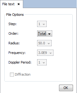
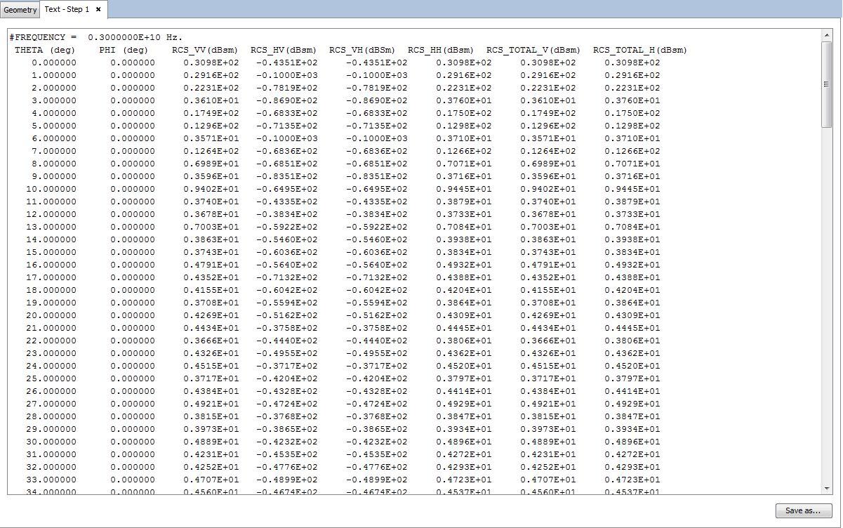
Step 19
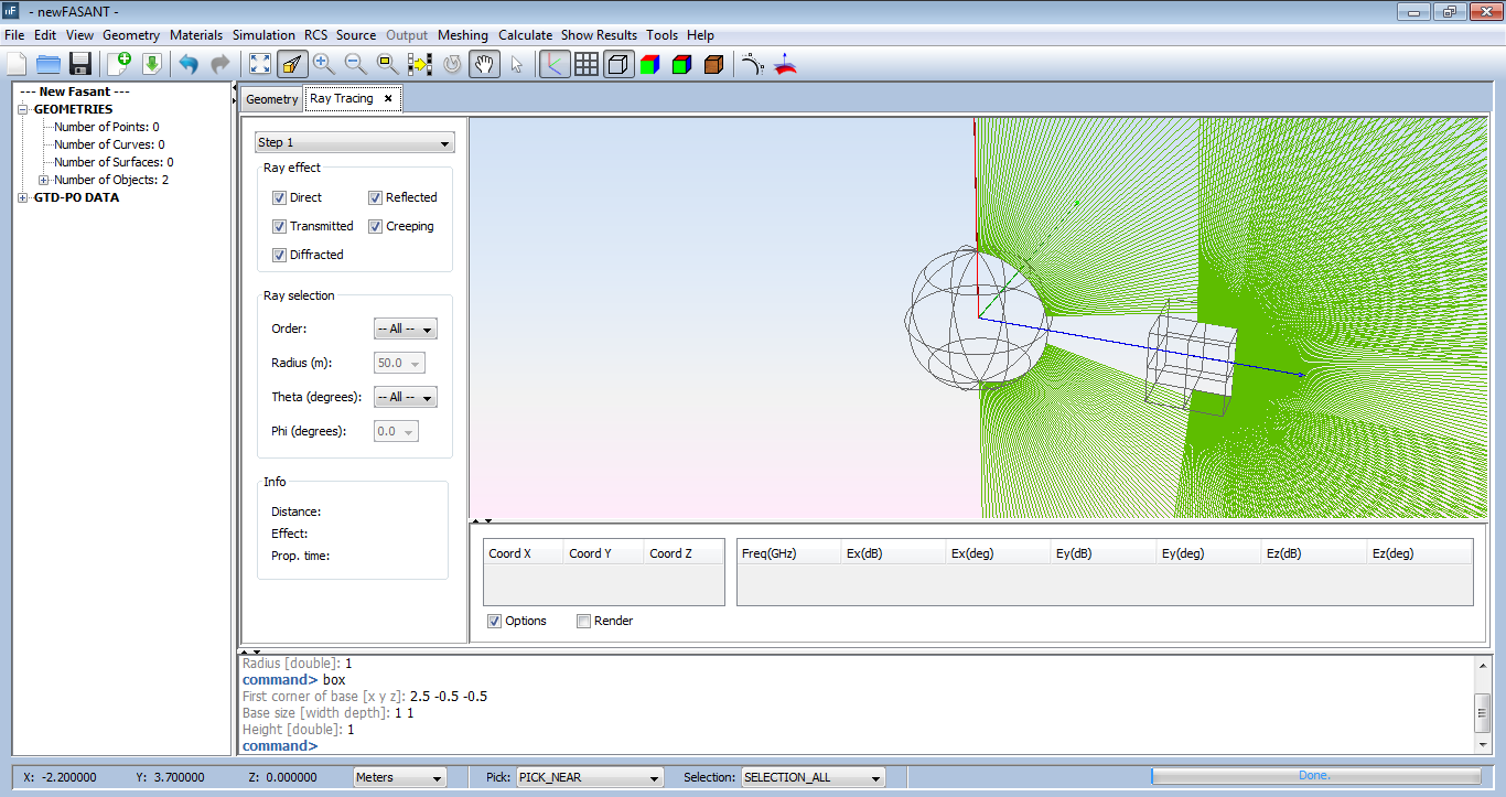
Click on Show Results → Ray Tracing → View Ray. It is possible to represent the ray tracing of the sources interacting with the geometry