Automotive RADAR
Calculate the electromagnetic signals observed by a moving automotive RADAR in traffic.
Model Type
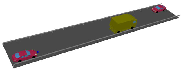
The car with the RADAR moves at 10 m/s and approaches the truck, which moves in the same direction at only 5 m/s. At the same time, a car approaches in the other lane, driving in the opposite direction at 10 m/s.
Sites and Antennas
The radar antenna has a forward-looking beam. It was generated in Altair Feko by simulating a simple array antenna and exporting the pattern in .ffe format. In ProMan, it was specified that the transmitter moves with the car. On the Edit Project Parameter dialog, click Sites. Edit the site to open the Cell dialog. Under Location of antenna, select the Transmitter is moving with group check box.
The frequency of operation is 77 GHz. The results are computed at one point only, the point where the RADAR is located, and this point also moves with the car. On the Edit Project Parameter dialog, click Simulation. Add a point and on the Prediction Point dialog, select the Time variant location (non-stationary) check box and select the group with which the point is moving.
The pattern of the receiving antenna is also considered. On the Edit Project Parameter dialog, click the Propagation tab and under Consideration of Antenna Properties at Mobile Station, select the Consider Antenna of MS check box.
RunPro calculates the rays that reach the point of interest (taking the transmitter’s antenna pattern into account) and RunMS then takes the receiver’s antenna pattern into account.
In this example, the same antenna pattern and the same location are used for transmitter and receiver.
Computational Method
The simulation is done with the standard ray tracing model (SRT), taking scattering into account. The inclusion of scattering was enabled in WallMan in the material catalogue. That is an essential step in WallMan. In WallMan, click and on the Material Catalogue dialog, double-click on a material. On the Material properties dialog, under propagation phenomena, select the Compute Scattering check box.
The inclusion of scattering is important because edge diffraction is weak at 77 GHz and reflections are only observed from perpendicular surfaces. Hence, without scattering, some objects might escape detection.
Results
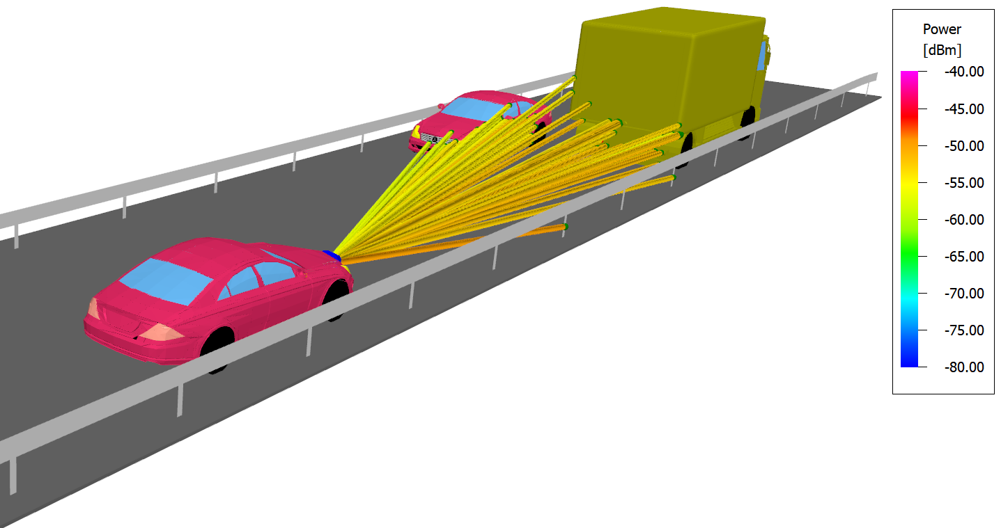
At every time step, WinProp reports the rays that reach the receiver, along with important properties: delay, signal level, and Doppler shift.
You can view the propagation paths to a selected receiver pixel by selecting Power or Power (MS) in the tree view and clicking . Click on a receiver pixel to view the Propagation Paths dialog.
All information is also written to a text file for further signal processing outside WinProp.