Example 9: Parameters, Frequency Sweep, Far and Near Field

This case explains how to generate a full example with most of options available in the tool geometric parameters, frequency sweep, primitive antennas, solver parameters, 3D radiation pattern, and observation entities for near field.

Step 1 Create a new MOM Project

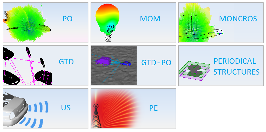
Open newFASANT and select File - New option. Select MOM on the module selection.

Step 2 Create the geometry

A quadri-filar helix antenna on a box which is moving according to a parameter will be generated.

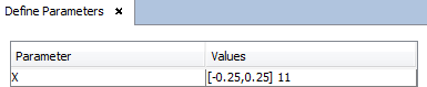
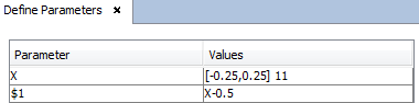
Create the geometric parameter to be used in the box later. Click on Geometry - Parameters menu and select the Define Parameters option. Then, click on Add parameter button and the new parameter added it is named X and its values ranges from -0.25 to 0.25 with 11 equispaced samples, as shown in next figure. Remember clicking on Save button before closing the parameters panel.

Figure 2. Parameter X defined

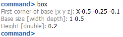
Now, create a box which is moving along the X axis according to the defined parameter. Tip box in the command line and press Enter key or click on Geometry - Solid menu and select the Box option. Define the box with the same arguments than shown below:

Figure 3. Box parameters

As the box definition contains an operation over the X parameter, a new auxiliary parameter has been added, so it is possible to use again this operation by repeating it or by using the name of this auxiliary parameter (in this example, it is named $1 but it may change in other cases). Verify that the auxiliary parameter has been correctly added within Geometry - Parameters - Define Parameters panel.

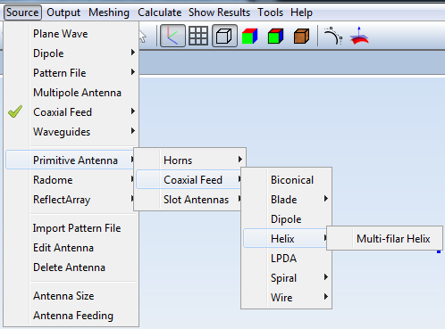
Now, an antenna will be placed on the top of the box in a fixed position. That means that only the box is moving. It may be useful to make a parametric study to find which is the optimal ground plane position for the antenna behaviour. Click on Source - Primitive Antenna - Coaxial Feed - Helix - Multi-filar Helix menu, as shown in the following figure.

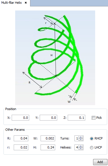
The Multi-filar Helix panel is open on right side. Set all parameters by default Z position, which is set to 0.1. Then, this primitive provide four ports defined one in each Helix. Confirm the antenna definition by clicking on Add button. After that, close the Multi-filar Helix panel.

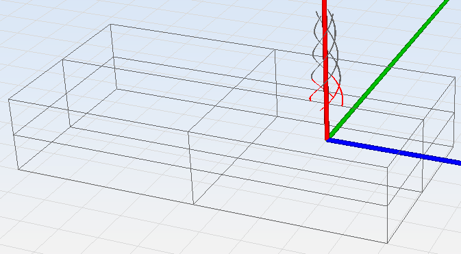
This antenna must be placed on a planar structure which acts as reference plane, so the box performs this function. The resulting geometry is represented in next figure.

Step 3 Set Simulation Parameters

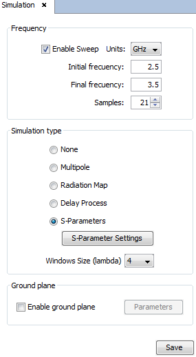
Click on Simulation - Parameters option on the menu bar. Set a Frequency Sweep and the None as shown in the figure below. Remember clicking on Save button to confirm the changes.

Note that a large number of frequencies has been set in this example, so the simulation time may requires several minutes due to the combination with the parametric steps. You may reduce the number of Samples to speed-up the simulation time and generate the example with less resolution.

Step 4 Set Solver Parameters

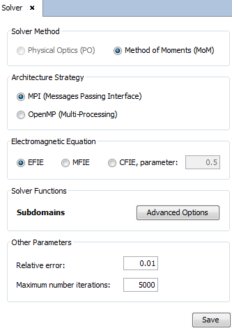
Click on Solver - Parameters option on the menu bar. Set the OpenMP Architecture Strategy, and then verify that all the parameters are defined by default, as shown in figure below.

Note that EFIE is set even having a box which is closed and could be analyzed with CFIE. As it is not an electrically large case and the convergence is good, we can solve it directly with EFIE. However, if CFIE is selected, the user must assign EFIE to the helix antenna within the Solver - Advanced Options - Specify.

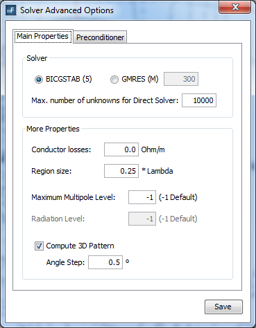
This example will be solved with Direct Solver. To do that, click on Advanced Options, and set the Max. Number of unknowns for Direct Solver with a value which is higher than the number of unknowns of the problem. As it is a small case, a value of 10000 is high enough for considering the Direct Solver. Note that the Compute 3D Pattern option is enabled, as we want to generate the 3D radiation pattern in the simulation process. Click on Save button to close the Solver Advanced Options window by confirming the changes.

Click on Save button before going to next step, and the Solver panel may be already closed.

Step 5 Output

Both Far field and Near field results are considered in this example.

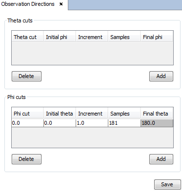
Regarding the Far field, click on Output menu and select the Observation Directions option. Set the default parameters in the Observation Directions panel, and click on Save button before closing it.

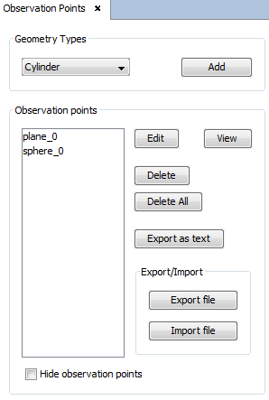
On the other hand, a plane and a progressive radial sphere will be generated as observation points. Click on Output menu and select the Observation Points option to open the Observation Points panel.

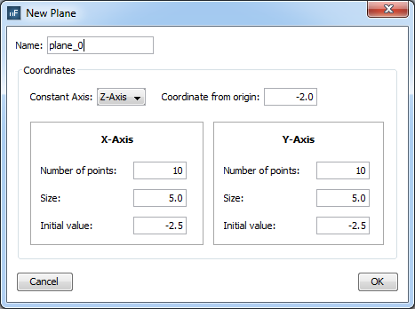
First, within the Geometry Types section select the Plane on the list and click on Add button to open the New Plane window. Set the values as shown in figure below and click on OK button to add the observation plane.

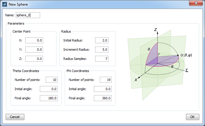
Next, within the Geometry Types section select the Sphere on the list and click on Addbutton to open the New Sphere window. Set the values as shown in figure below and click on OKbutton to add the observation sphere. Note that several Radius Samples has been set, so we will generate multiple spheres in the same entity and the Radial Points results will be enabled after the simulation process.

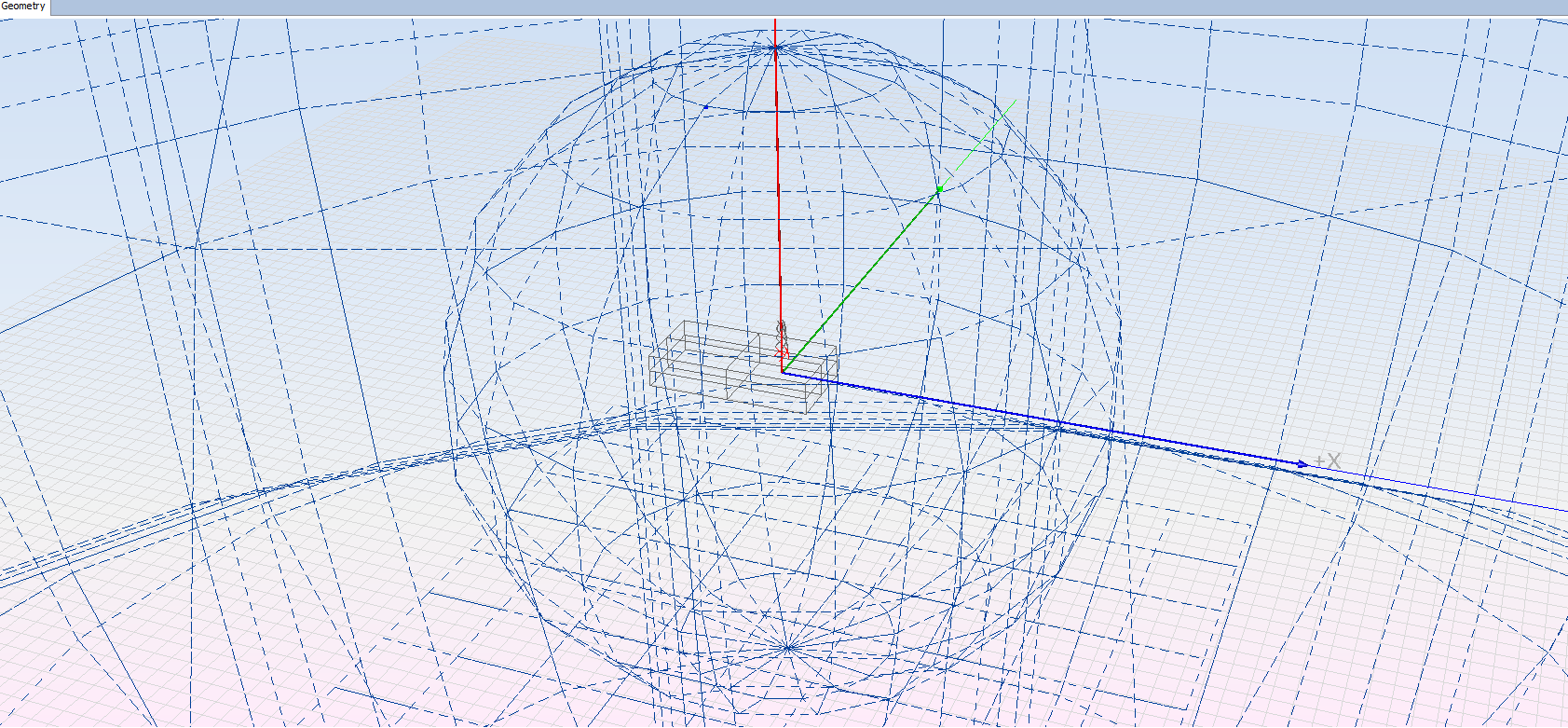
Having inserted the plane and the sphere as observation points entities, they are shown together the geometry in the Geometry panel. Then, you can close the Observation Points panel.

Step 6 Meshing

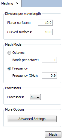
Click on Meshing - Create Mesh option on the menu bar. To use the same mesh for all the frequency sweep, select the Frequencyand specify the upper frequency of the range, 0.9 GHz. Select the available number of Processors, and then launch the meshing process by clicking on Mesh button.

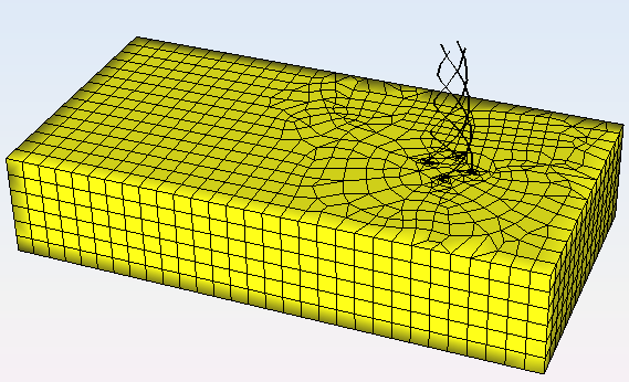
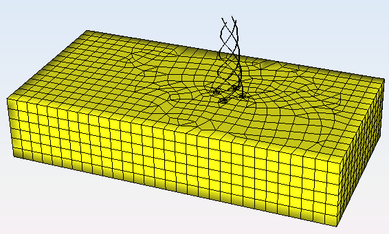
After the end of the meshing process, the meshes may be visualized by clicking on Meshing - Visualize Existing Mesh and select the mesh in any frequency folder within the desired step folder. Then, you can verify that the mesh show the electrical continuity between the helix filaments and the box, as shown in next figure.

Step 7 Execute

Click on Calculate - Execute menu and launch the simulation with the available processors. Launch the simulation by clicking on Calculate button.

Step 8 Results

When the simulation process has finished, most of options are enabled within the results menu.

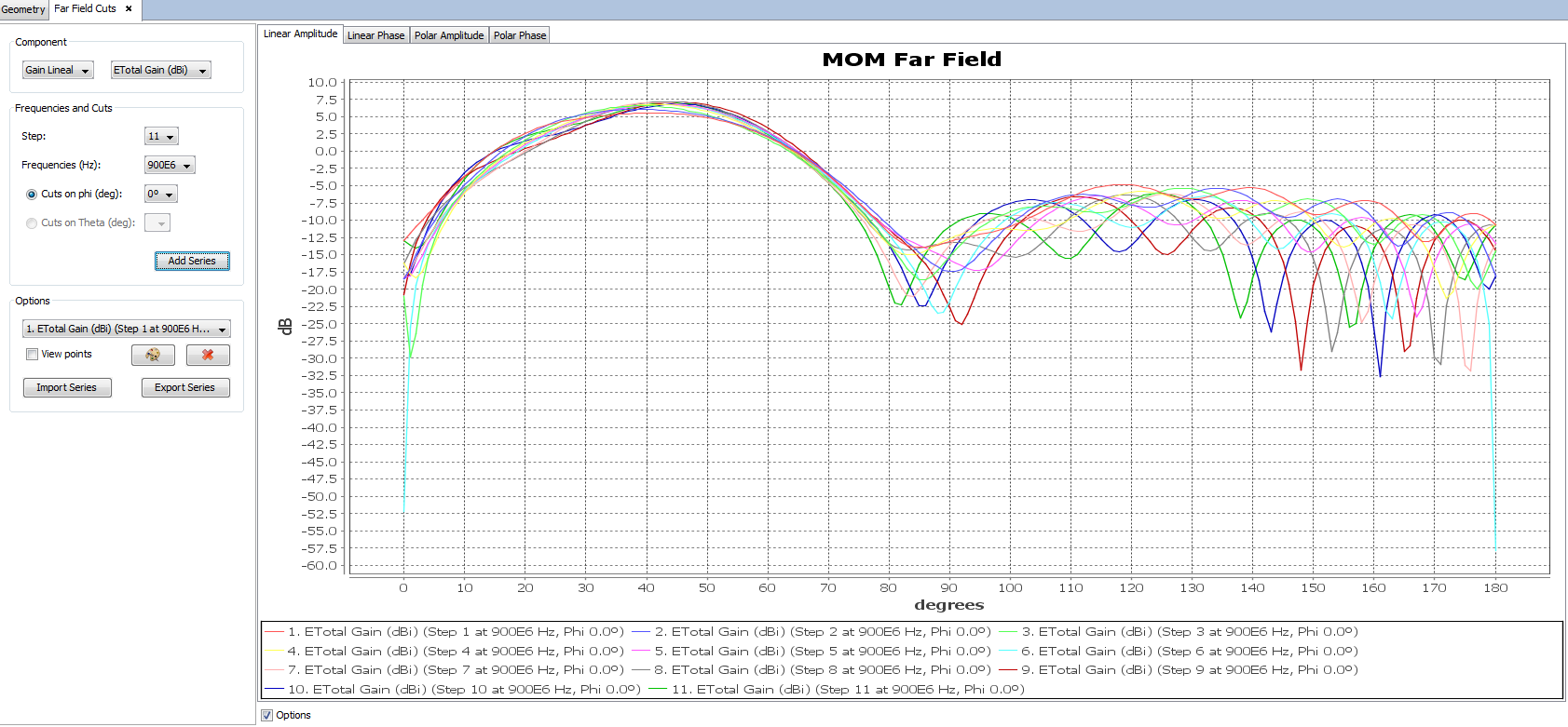
Click on Show Results - Far Field menu and View Cuts option. In the figure below, we compare the Total Gain of the only considered far field cut versus all the geometric steps. To do that, select the Gain Lineal - ETotal Gain, and then click on Add Series button after selecting every step.

Click on Show Results - Radiation Pattern menu and View Cuts By Step option. In the next figure, a comparison of a far field direction (obtained from the 3D radiation pattern) versus the parametric step is shown. To do that, select the Circular, and then click on Add Series button after selecting each component.

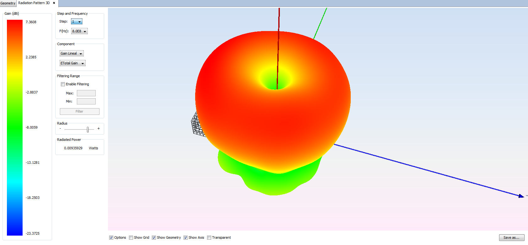
To visualize the 3D radiation pattern, click on Show Results - Radiation Pattern menu and View 3D Pattern option. The diagram of the first parametric step at 800 MHz is depicted in next figure.

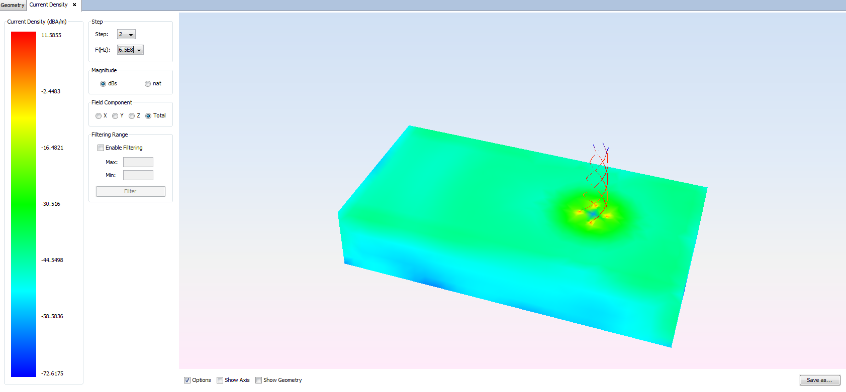
The next figure shows the current distribution on the structure at the second parametric step. To visualize it, click on Show Results - View Currents menu.

Far field 3D pattern

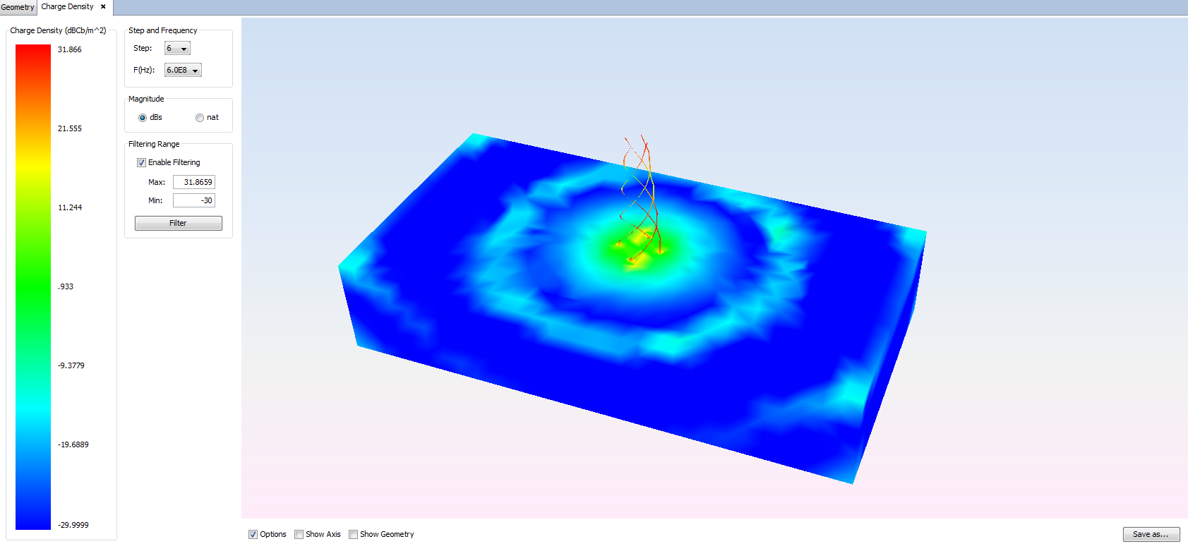
The charges density on the structure is represented in next figure. To visualize it, click on Show Results - View Charges menu. Note that the Enable Filtering has been enabled.

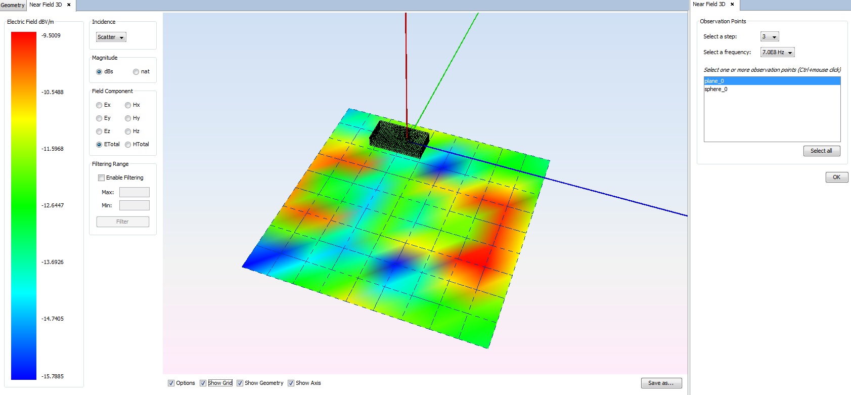
The next figure shows the near field distribution on the observation plane. To visualize it, click on Show Results - Near Field menu and select the first option, View Near Field Diagram. Then, select the Step, Frequency and Observation entity in the Near Field 3D panel and click on OK button to open the results.

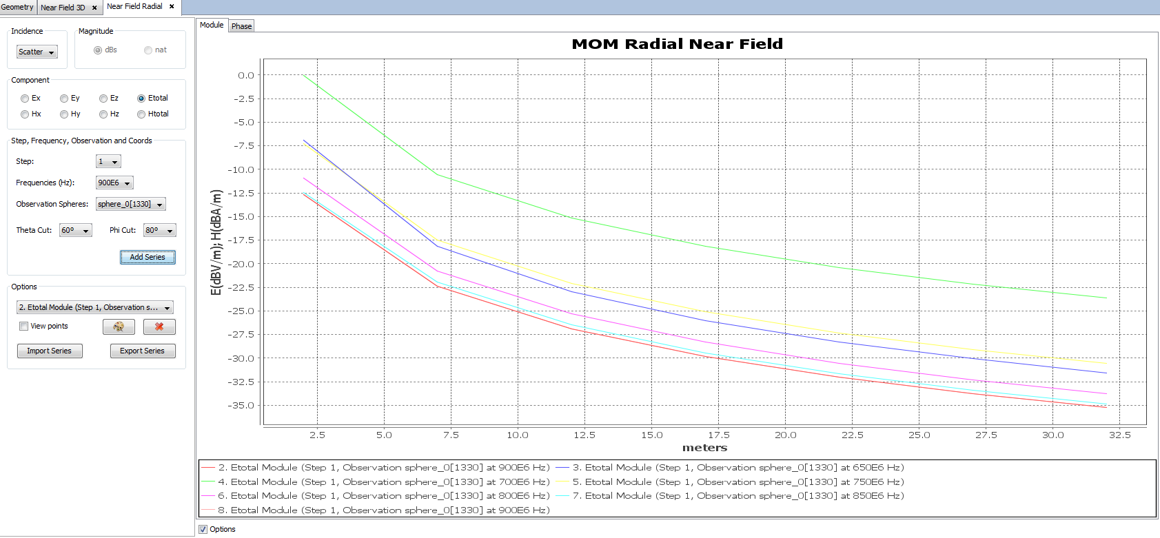
The last results represented in this example is the Near field obtained from the observation radial spheres in a near field direction at all the simulated frequencies. To do that, Click on Show Results - Near Field menu and select the View Radial Points option. To do that, select the Theta and Phi directions, and then click on Add Series button after selecting frequency step.