Tutorial Level: Beginner Learn about the Inspire Extrude Interface, set up and complete a solid profile
extrusion analysis, and post-process the results for interpretation.
Open the Tutorial Model
Before you begin, copy the file(s) used
in this tutorial to your working directory.
Browse to your working directory, select
RubberTrimSolid.x_t, and click
Open.
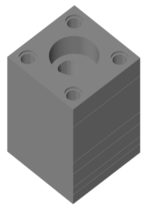
The model should appear in the Inspire Extrude window.
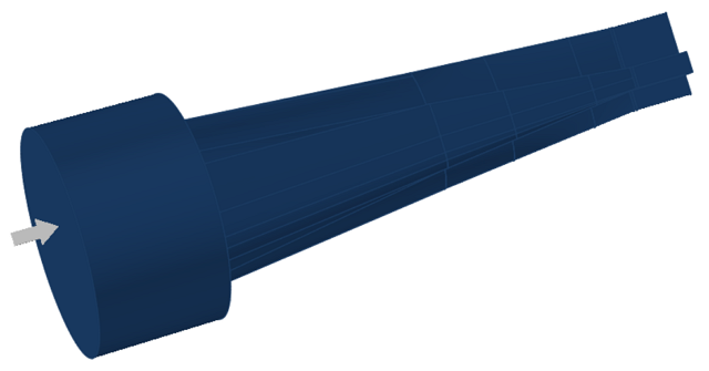
Orient the Model
Click the Polymers ribbon.
Click the Orient icon.
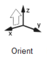
On the model, click the exit surface.
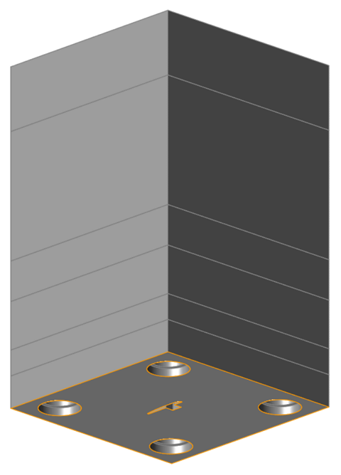
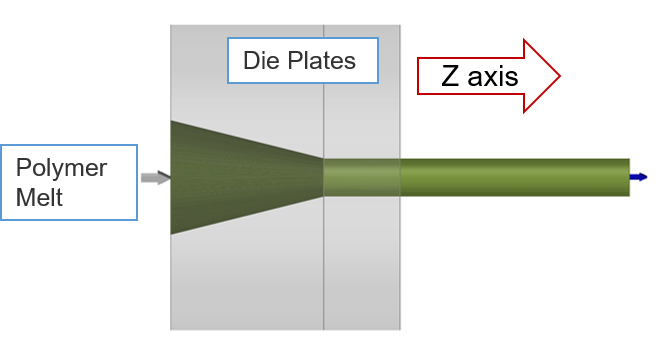
The model is oriented such that the profile is on the run-out table
surface, which is at Y=0, and the profile extrudes in the +Z direction.
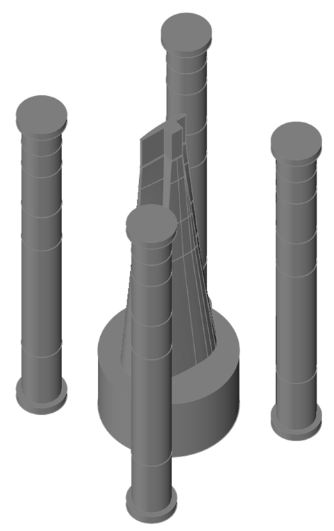
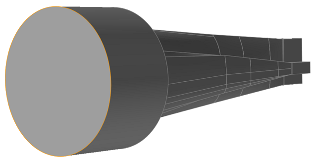
Extract Flow Volume
Click the Polymers ribbon.
Click the Flow Volume icon.
Click and drag the cursor over the whole model to create a box select, then
release.
Delete Unwanted Solids
Orient the model such that selecting solids is easy.
Select solids which belong to Flow Volume and hide them by pressing
H.
Delete the remaining solids.
Press A to reveal the remaining solids.
Hold CTRL and select multiple solids on the exterior of
the model.
Press H to hide the selected solids.
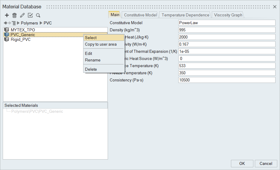
Select Materials
Click the Materials icon.
Select PVC > PVC_Generic
Right click on the alloy name and select it.
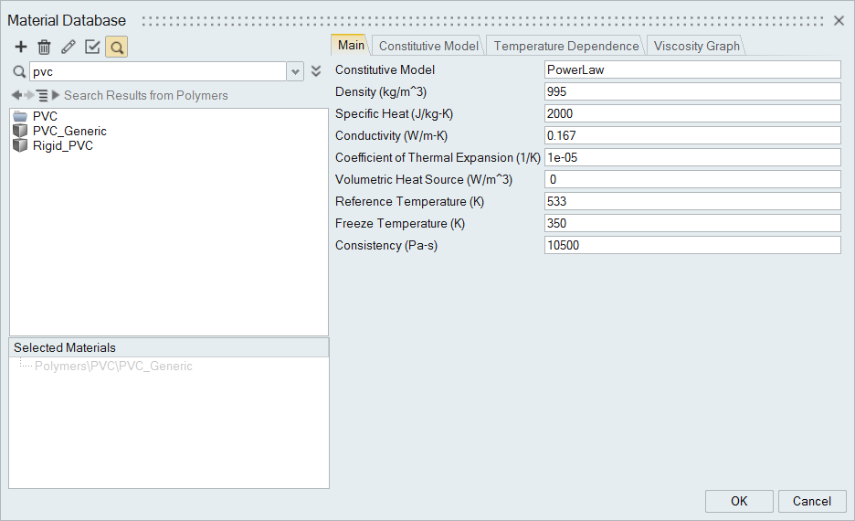
Note: Another way to search for your materials is to click in the search box in the
materials window.
Click in the search box.
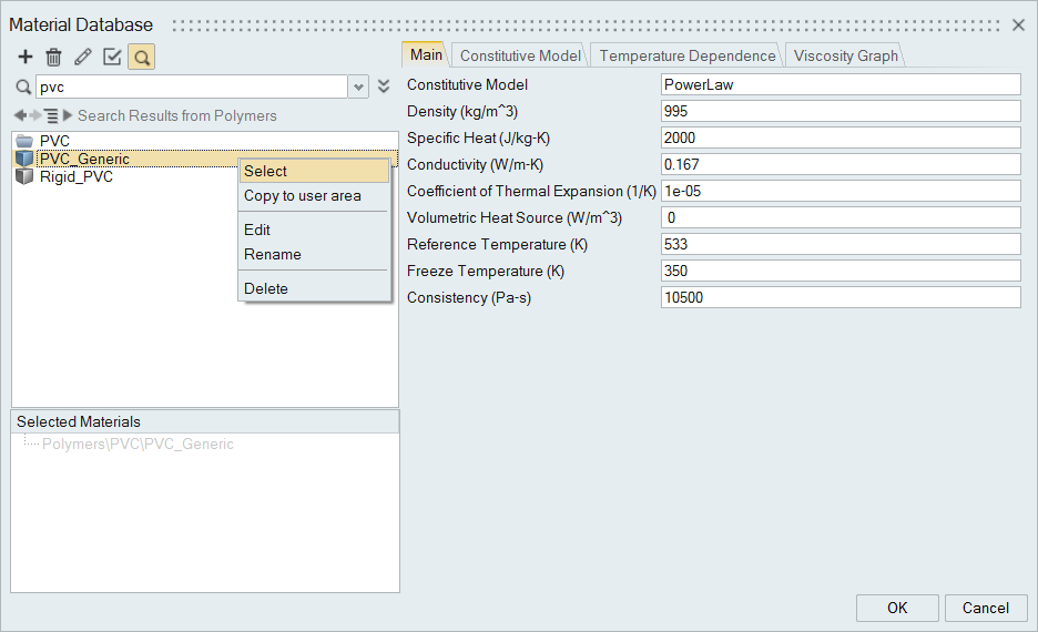
Type the name of the alloy.
Right click on the alloy name and select it.
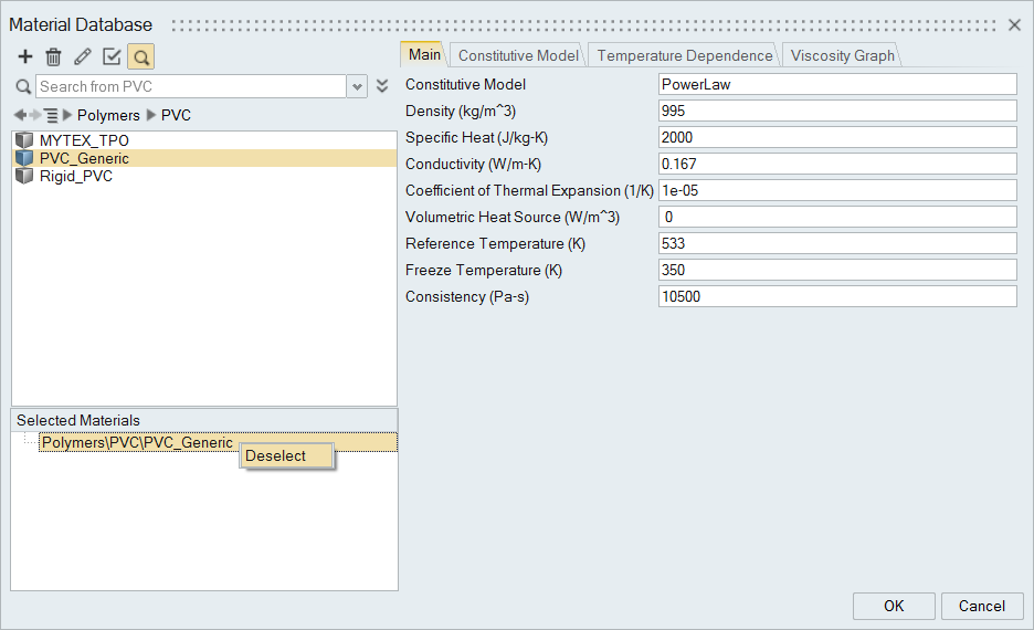
Note: You can deselect a material by right-clicking on a selected material and
clicking Deselect. This is a single polymer extrusion
die, so you only need one polymer for this simulation.
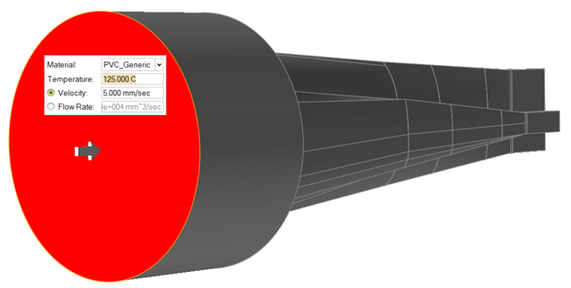
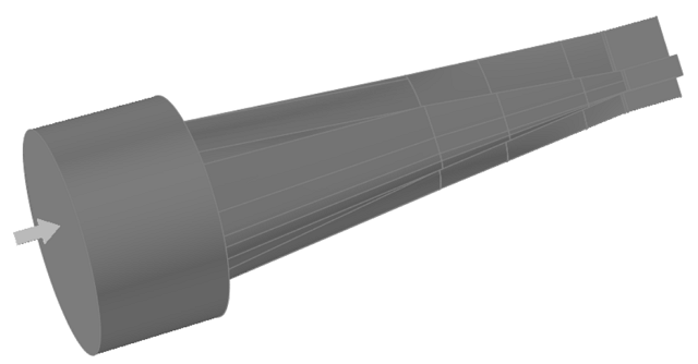
Specify Process Data - Inlet
Click the Inlet icon.
Zoom in to the inlet region of the polymer melt and select the inlet face.
Specify the inlet conditions.
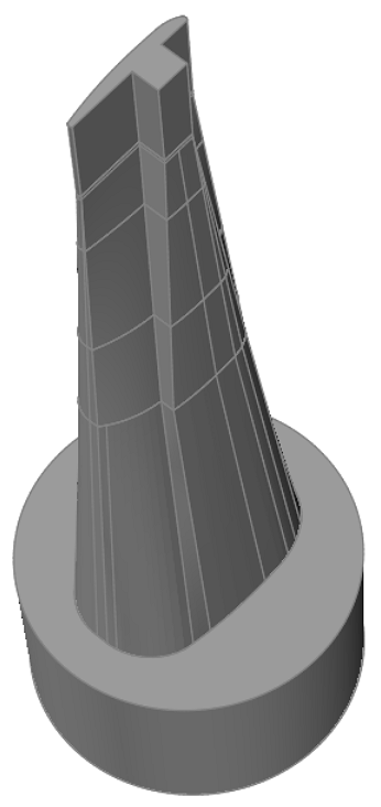
Organize Solids into Polymer Layers
Display only flow solids which define the polymer flow.
Click the Organize icon.
Inspire Extrude will combine the required solids, rename,
and organize the selected solids to the Layer-1 assembly.
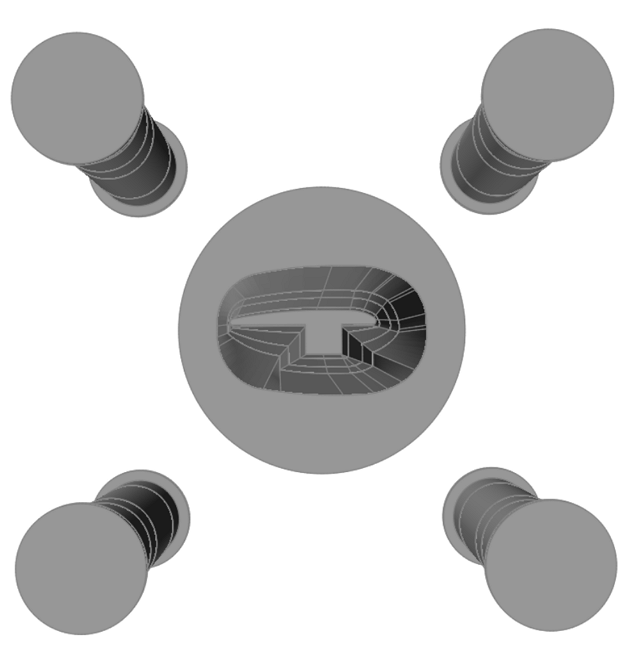
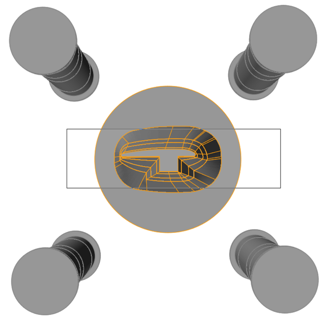
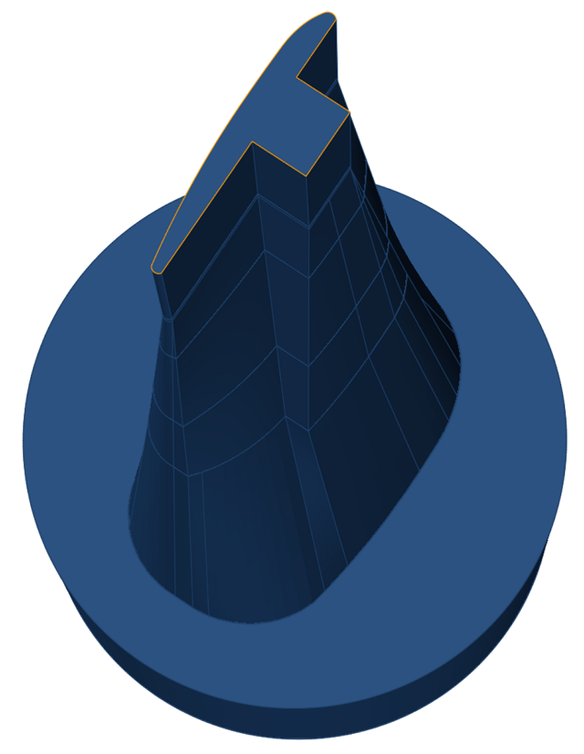
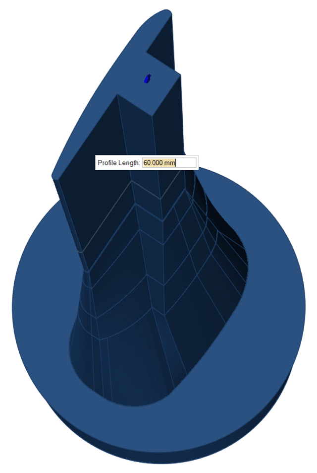
Create Profile Solids
Click the Profile icon.
Zoom in to the land surface as shown and click on that surface.
Inspire Extrude will create a Profile solid and use 3 times the
length of Land as its default. You can change this as needed. This model
requires a 60mm Profile solid length. There is only one exit in this model, so
you do not need to repeat this step.
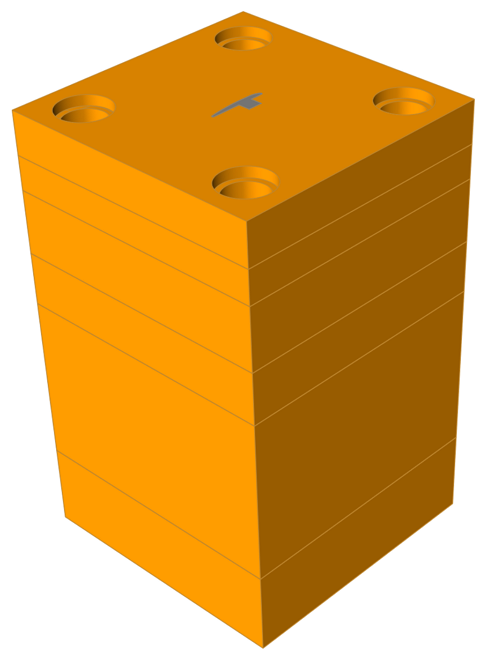
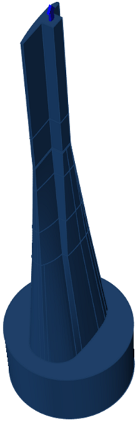
Delete Die Assembly Solids
Select die plate solids that belong to the die assembly and delete them as
shown. Reveal them by pressing A. These solids are not
required for flow simulation and create issues in geometry cleanup.
Save the Model
Click File > Save As... to save the model.
Note: We suggest you save this new model in a location that is different than
the original tutorial model's location to prevent any future conflict with
those files.
Submit the Job for Simulation
Click the Run Analysis icon.
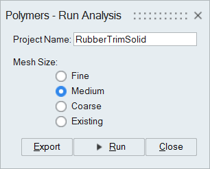
Specify parameters for the analysis process.
Click Run.
Monitor Job Status
Once the results are ready, you should see a green flag above the
Analysis icon notifying you that the results are
ready for visualization.
Interpret Out File Data
The goal of post-processing is to interpret the results generated by the solver and
apply them to validate/improve the design. Results generated by the solver are stored
in two key files:
Out file: This is an ASCII file, which helps to verify the input data and gives a
quick overview of the result.
H3D File: This is a Binary file with detailed results.
Note: Even though this section is built off the results from this specific tutorial, it
has general applicability throughout any project in Inspire Extrude.
Verify the Input data by checking these pieces of data:
Solution Convergence
Mass Balance Table
Min/Max Velocity Table
Force Balance Table
Energy Balance Table
Solution Summary
Extrusion Ratio: Check if the extrusion ratio is correct by checking
these aspects of the model:
Check the ratio of the inlet to the exit area, which gives an overall
measure of how much material deforms during extrusion.
If the value of the extrusion ratio is incorrect, inspect the inflow and
outflow boundaries in the model to verify and correct them.
License Type: Depending on what problem type you are solving, a basic or
advanced license will be checked out.
Model Information: Check the analysis information by verifying these
values:
Value 0 for Geometry indicates it is a 3D model.
Value 0 indicates that the Stokes equations are solved.
Value 0 indicates a non-isothermal analysis.
Value 1 indicates a steady Simulation.
The Review Unit system is under the MODEL UNITS
section.
Verify the Model information by confirming the following:
The tool material is denoted as Solid material.
The extruded material is denoted as Fluid material.
In this example, the tool analysis is NOT performed, so the number of
solid materials is 0.
Check the mesh size and type of elements.
Note: Most of these data are default values and are seldom modified by the
user.
Model Parameters: Verify the Mesh update parameters. To do so:
Check if the free surface calculation is performed.
Verify other related parameters such as free surfaces, star location,
etc.
Review Material Properties. To do so,
Verify the viscosity models employed for the polymer materials.
Verify the constitutive model data.
Verify how the temperature dependency of viscosity is accounted
for.
Reference Quanitities:
Examine the Energy Equation Data. Work is converted into energy (%), which
accounts for viscous dissipation. Check the reference quantities used in the
analysis. Verify different parameters used in the numerical solution. To do
so,
Look at the relaxation parameters used in the solver.
Look at the convergence criterion used for the solution variables.
Note: Most of these data are default values and are seldom modified by the
user.
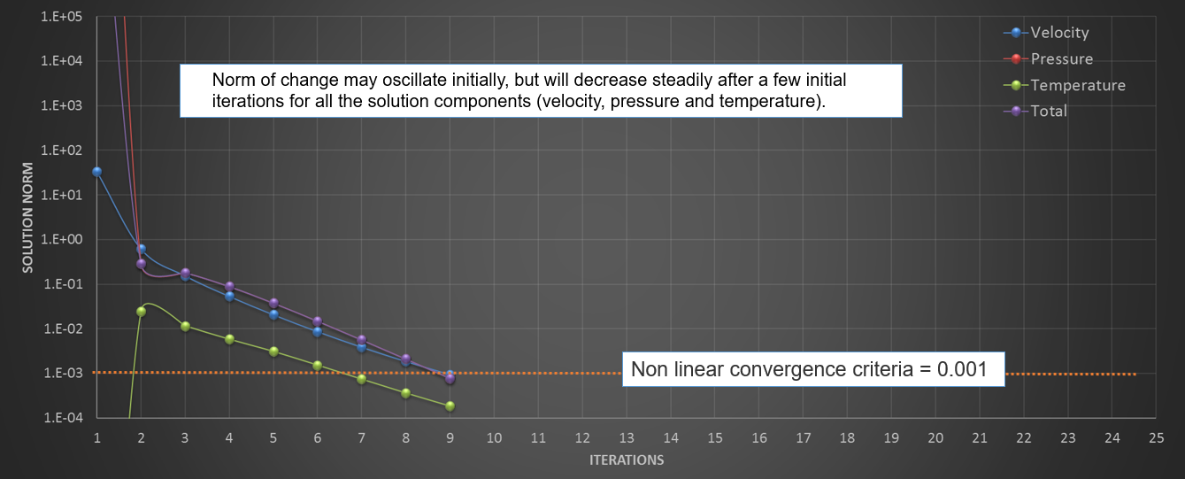
Solution Convergence History:
Check the Norm of Change in the Solution. The Norm of Change may oscillate
initially, but it will decrease steadily after a few initial iteration for all
of these solution components: Velocity, pressure, and temperature. The solution
is considered 'converged' if the value of the Norm of Change in the Solution is
less than the tolerance (0.001) for all of the variables. A slow convergence
rate or oscillatory behavior indicates that the mesh is too coarse.
Note: The
plot is created using data in the converge.hist file.
Verification of Mass Balance:
Check if the Mass Balance is less than 1% to ensure conservation of mass. The
Mass Flux table shows mass flow rate across each boundary. A positive sign
indicated material entering through the boundary, and a negative sign indicates
material leaving the boundary.
Average Velocity:
The table also shows average velocity of the material entering/leaving through
each boundary surface. Note that velocity on a solid wall must be close to zero
and velocity on symmetric planes must be equal to 0. Velocity on free surface
boundaries must be small - at least a few orders of magnitude less than
extrusion speed.
Min/Max Velocities:
The Profile exit velocity in the extrusion direction must be significantly
higher than the velocity in other directions. Velocities in directions other
than the extrusion direction indicate the possibility of profile deflection.
Velocities at the solid wall must be close to zero.
Verification of Force Balance:
A positive sign indicates force that is applied on a surface, and a negative
sign indicates response The table also contains the average pressure at
each boundary surface.
Check if the average pressure at the inlet is within
the acceptable range. Verify the boundary
conditions and material properties if the check fails.
Viscous Dissipation:
The amount of heat generated during deformation should only have up to a 5%
divergence from the mechanical work's heat output. The above number can be computed from the pressure on the inlet
face, inlet velocity, area of the inlet face, and the % of work converted to
heat. Some examples are as follows:
P = 10 MPa = 10 e+6 Pa
V = 5 mm/s = 0.005 m/s
A = 4000.0 mm^2 = 4000e-6 m^2
% conversion = 90%
Heat Generated = 10e+6 X 0.005 X 4000e-6 x 0.9 = 187.55W = 180 W = 0.180
kW. The value of viscous dissipation from the Heat Balance table = 1.81e-1 kW.
The difference is less than 5%
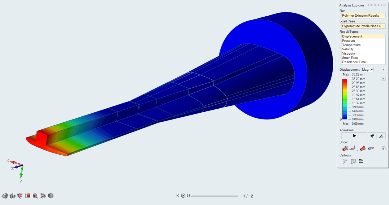
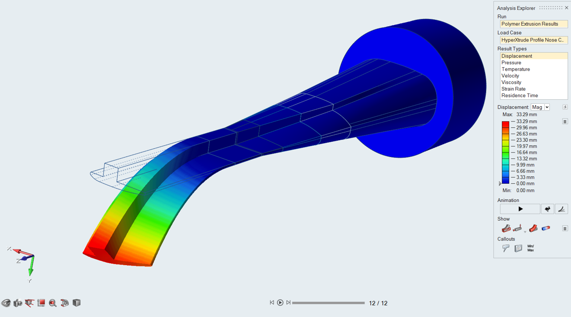
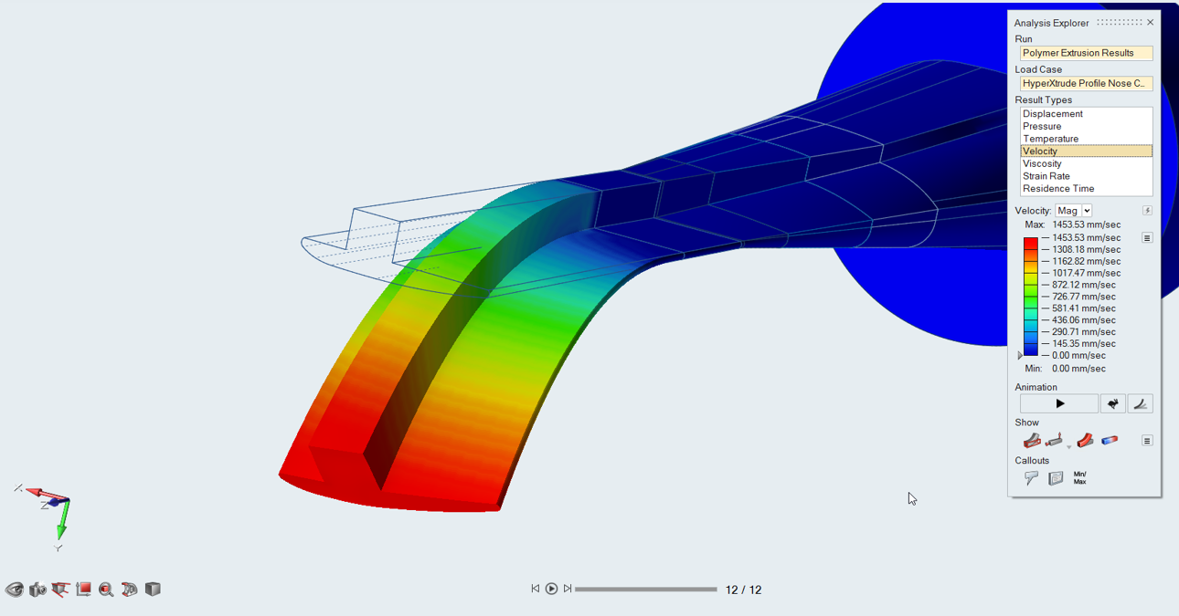
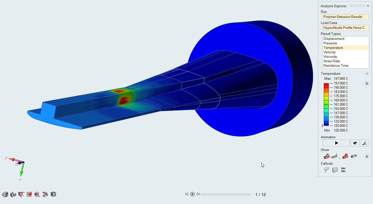
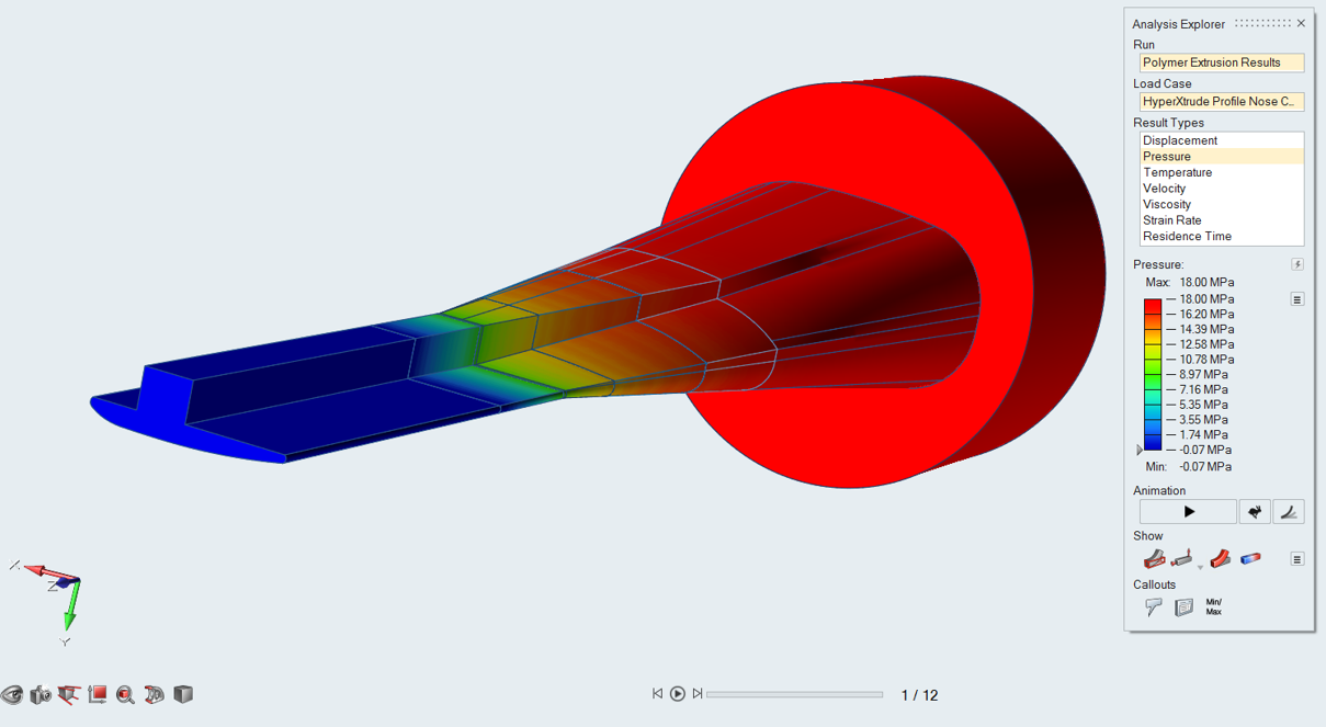
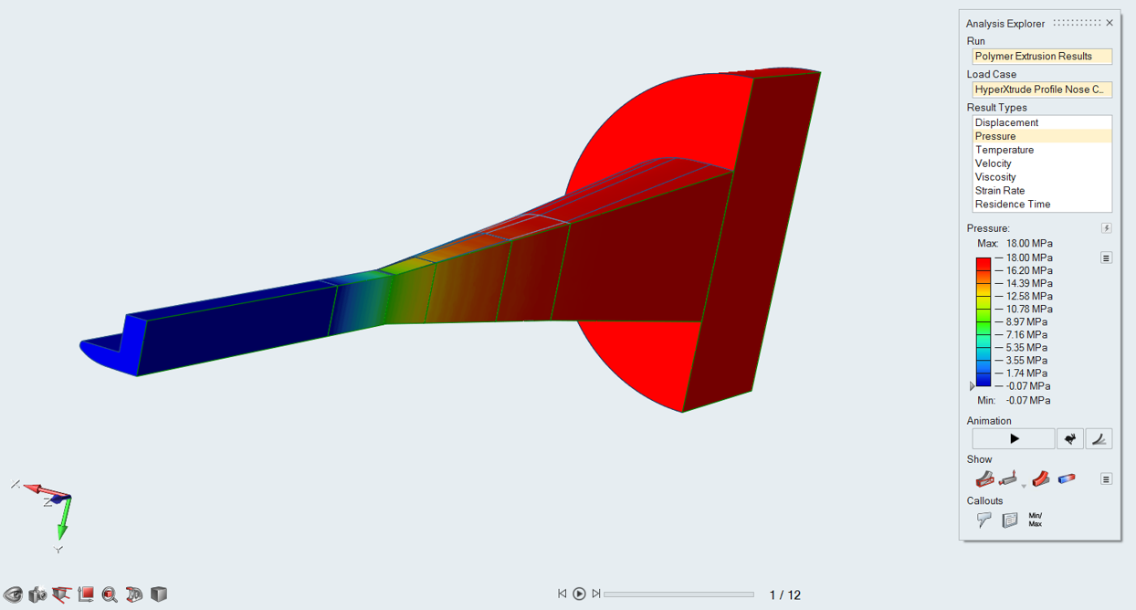
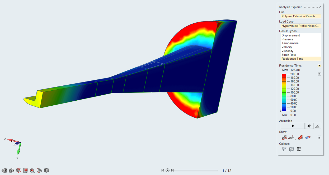
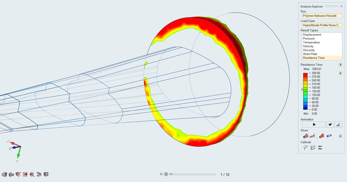
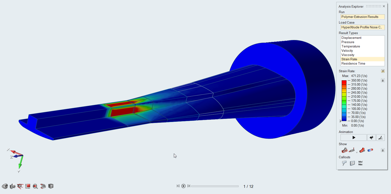
View Simulation Results
Review simulation results in the Analysis
Explorer.