RD-V: 0030 Spring (TYPE4)
Spring force as function of elongation for different stiffness formulations.
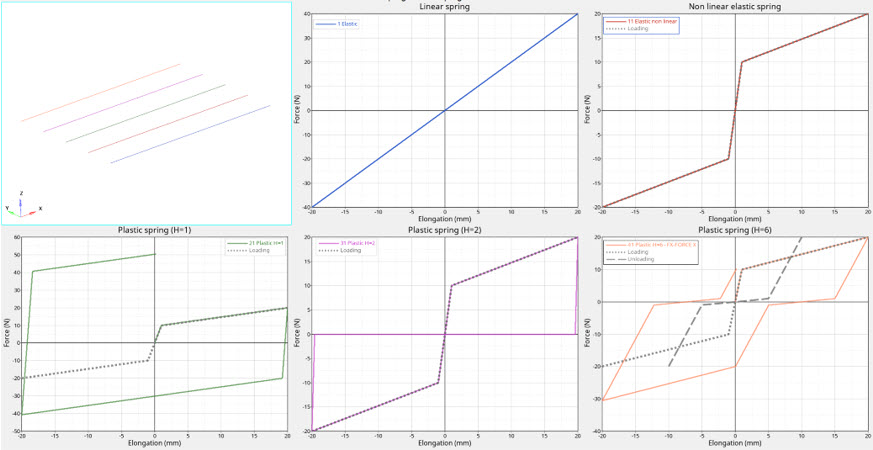
Figure 1. Force versus elongation
The subject of this study is to verify the behavior of the spring element using different stiffness formulations with a defined elongation.
Options and Keywords Used
Input Files
Model Description with Different Stiffness Formulation
Units: Mg, s, mm, MPa
- Elastic linear stiffness
- K=2N/mm
- Nonlinear elastic stiffness
- Force versus displacement function:
- Elongation
- Force
- -20
- -20
- -1
- -10
- 0
- 0
- 1
- 10
- 20
- 20
- Linear stiffness K=50N/mm used for transition
- Force versus displacement function:
- Nonlinear plastic stiffness with isotropic hardening
(H=1)
- Same force versus displacement function and same linear stiffness
- Plastic behavior with H=1
- Linear stiffness K=50N/mm used for transition
- Nonlinear plastic stiffness with uncoupled hardening
(H=2)
- Same force versus displacement function and same linear stiffness
- Plastic behavior with H=2
- Linear stiffness K=50N/mm used for transition
- Nonlinear plastic stiffness with nonlinear unloading
(H=6)
- Same force versus displacement function and same linear stiffness
- Nonlinear unloading force versus displacement:
- Elongation
- Force
- -10
- -20
- -5
- -1
- 0
- 0
- 5
- 1
- 10
- 20
- Plastic behavior with H=6
- Linear stiffness K=50N/mm used for transition
Imposed displacement is defined on one end of the spring element to model tensile and compression (displacement +/- 20mm) with constant velocity of 200mm/s.
The other end of the spring element is clamped.
Results
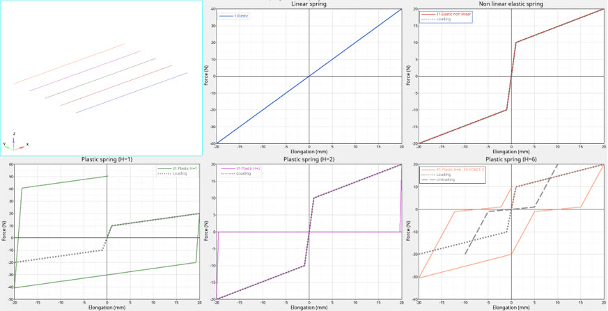
Figure 2. Force versus elongation
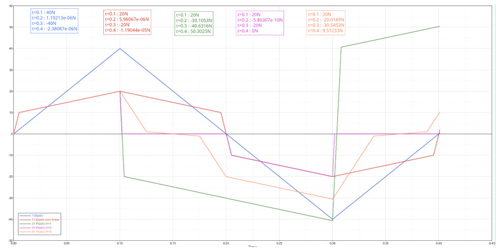
Figure 3. force versus time
| Time | Elastic Linear Stiffness | Nonlinear Elastic | Nonlinear Plastic Stiffness with Isotropic Hardening (H=1) | Nonlinear Plastic Stiffness with Isotropic Hardening (H=2) | Nonlinear Plastic Stiffness with Nonlinear Unloading (H=6) |
|---|---|---|---|---|---|
| t=0.1s | 40 | 20 | 20 | 20 | 20 |
| t=0.2s | 0 | 0 | -30.10526316 | 0 | -20 |
| t=0.3s | -40 | -20 | -40.63157895 | -20 | -30.52631579 |
| t=0.4s | 0 | 0 | 50.30249307 | 0 | 9.473684211 |
Model Description with Behavior at Different Deformation Rates
Units: Mg, s, mm, MPa
- Nonlinear elastic stiffness
- Force versus elongation function:
- Elongation
- Force
- -20
- -20
- -1
- -10
- 0
- 0
- 1
- 10
- 20
- 20
- Force versus elongation function:
- Elongation rate dependency
- Linear value
- Stiffness scale factor
- Force versus elongation rate scale factor function:
- Elongation Rate
- Force
- -10
- 0.1
- 0
- 0
- 10
- 0.1
- Damping versus elongation rate function
- Elongation Rate
- Damping
- -10
- -1
- 0
- 0
- 10
- 1
- Damping versus elongation rate function with higher velocity
The imposed displacement function abscissa (time) is scaled by 0.5 to double the constant loading velocity.
Imposed displacement is defined on one end of the spring element to model tension and compression (displacement +/- 20mm) with constant velocity of 200mm/s (with abscissa scale factor 1.0) or 400mm/s (with abscissa scale factor 0.5).
The other end of the spring element is clamped.
Results
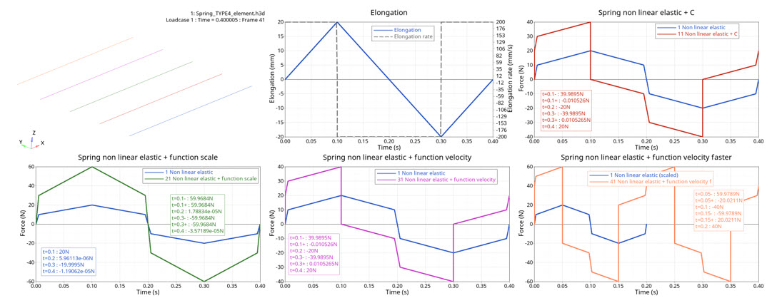
Figure 4. force versus time
| Time | Nonlinear Elastic | Nonlinear Elastic + C | Nonlinear Elastic + Velocity-based Force Function Scale | Nonlinear Elastic + Velocity-based Damping Function (200 mm/s) | Nonlinear Elastic + Velocity-based Damping Function (400 mm/s) |
|---|---|---|---|---|---|
| t=0.1s (V+) | 20 | 40 | 60 | 40 | 60 |
| t=0.1s (V-) | 20 | 0 | 60 | 0 | -20 |
| t=0.2s (V-) | 0 | -20 | 0 | -20 | -40 |
| t=0.3s (V-) | -20 | -40 | -60 | -40 | -60 |
| t=0.3s (V+) | -20 | 0 | -60 | 0 | 20 |
| t=0.4s (V+) | 0 | 20 | 0 | 20 | 40 |
Conclusion
The Radioss computation returns results very close to the theoretical values with the expected behavior for the different elastic, plastic behavior and with deformation rate formulations.