Tutorial Level: Advanced This tutorial demonstrates a cellular phone drop test simulation using explicit analysis
in OptiStruct.
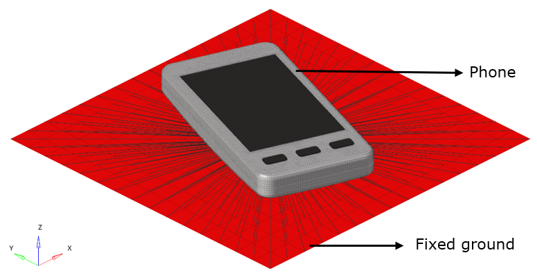
Figure 1 illustrates the structural model used for this tutorial; the phone and its parts
are considered in this model. The phone is dropped on the floor with a velocity of
5425 mm/s. Figure 1. Model and Loading Description
Before you begin, copy the file(s) used in this tutorial to your
working directory.
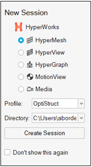
In the New Session window, select HyperMesh from the list of tools.
For Profile, select OptiStruct.
Click Create Session.
Figure 2. Create New Session This loads the user profile, including the appropriate template, menus,
and functionalities of HyperMesh relevant for
generating models for OptiStruct.
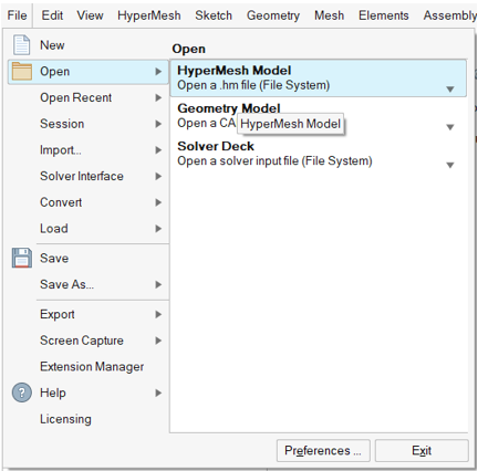
Open the Model File
On the menu bar, select File > Open > HyperMesh Model.
Navigate to and select the Drop_test_phone.hm file saved in your
working directory.
Click Open.
The Drop_test_phone.hm database is loaded into the current
HyperMesh session, replacing any existing
data.Figure 3. Model Import Options
Tip: Alternatively, you can drag and drop the file onto the
viewport from the file browser window.
The database
contains meshed data, contact definitions, and control
cards.
Set Up the Model
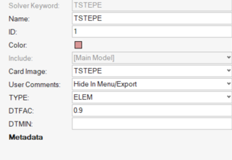
Create a Load Collector for TSTEPE
In this step, the time-step control parameters for explicit analysis is defined.
In the Model Browser, right-click and select Create > Load Collector.
If the Model Browser is not open by default, you can
open it from the menu bar by clicking View > Model Browser.
For Name, enter TSTEPE.
Select a color from the color palette.
For Card image, select TSTEPE from the drop-down
menu.
For Type, select ELEM.
For DTFAC, enter 0.9.
Figure 4. TSTEPE Definition
Click Close.
Create a Load Collector for SPC
In this step, Single Point Constraints (SPCs) are used to fix the floor.
In the Model Browser, right-click and select Create > Load Collector.
For Name, enter SPC.
The load collector SPC is automatically made current as it was the most
recently created. If it is not, you can right click on
SPC and select Make
Current.
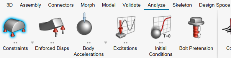
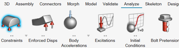
Open the Analyze ribbon.
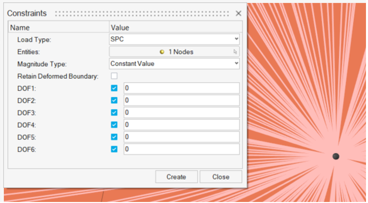
Click Constraints.
Figure 5. Constraints Tool
For Entities, select Nodes.
Rotate the model over to the underside of the floor and select the independent
node (center node) of the RBE2 element (see Figure 6).
Click .
Select all DOF check boxes (1, 2, 3, 4, 5, 6) and enter a value of
0.
This indicates all degrees of freedom are fixed.Figure 6. Definition of SPC on Selected Node
Click Create.
Click Close.
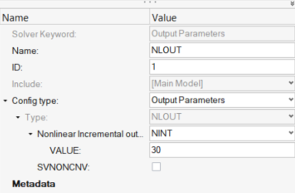
Create Load Step Inputs for NLOUT
In the Model Browser, right-click and select
Create > Load Step Inputs.
For Name, enter NLOUT.
For Config type, select Output Parameters from the
drop-down menu.
The default type is NLOUT.
For Nonlinear Incremental output, select NINT from the
drop-down menu.
For VALUE, enter 30.
Figure 7. NLOUT Definition
Click Close.
Create a Load Collector for Initial Velocity
In this step, an initial velocity of 5425 mm/s is applied to the phone in the
negative Z direction.
In the Model Browser, right-click and select Create > Load Collector.
For Name, enter INI_VEL.
Click Close.
On the Analyze ribbon, click Constraints.
Figure 8. Constraints Tool
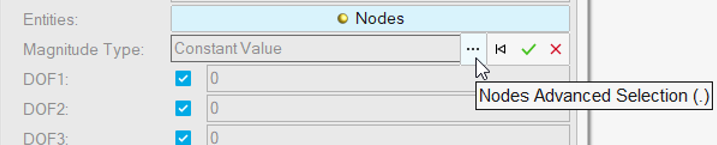
For Load type, select TIC(V).
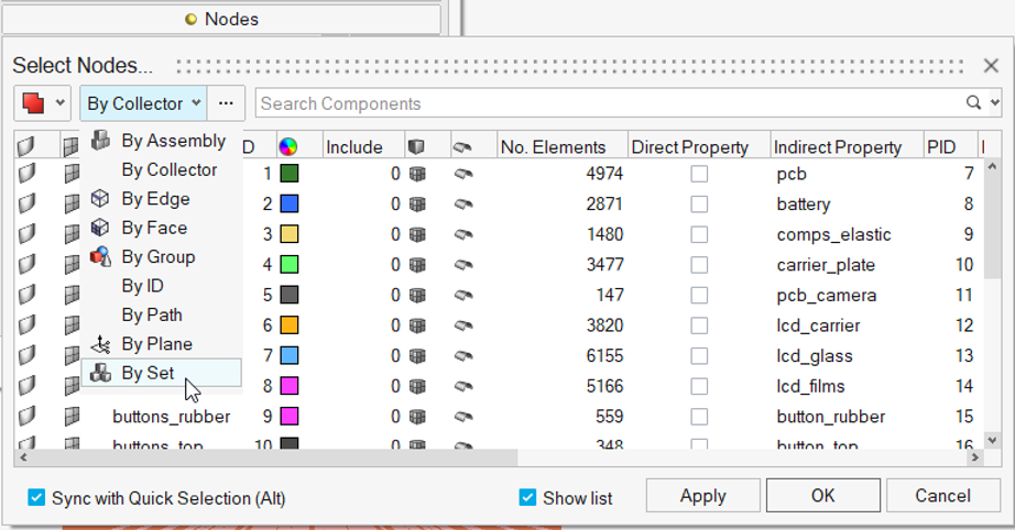
For Entities, select Nodes > to open Advanced Selection.
Figure 9. Open Advanced Selection
For selection type, from the drop-down menu select By
Set.
Figure 10. Select Nodes by Set
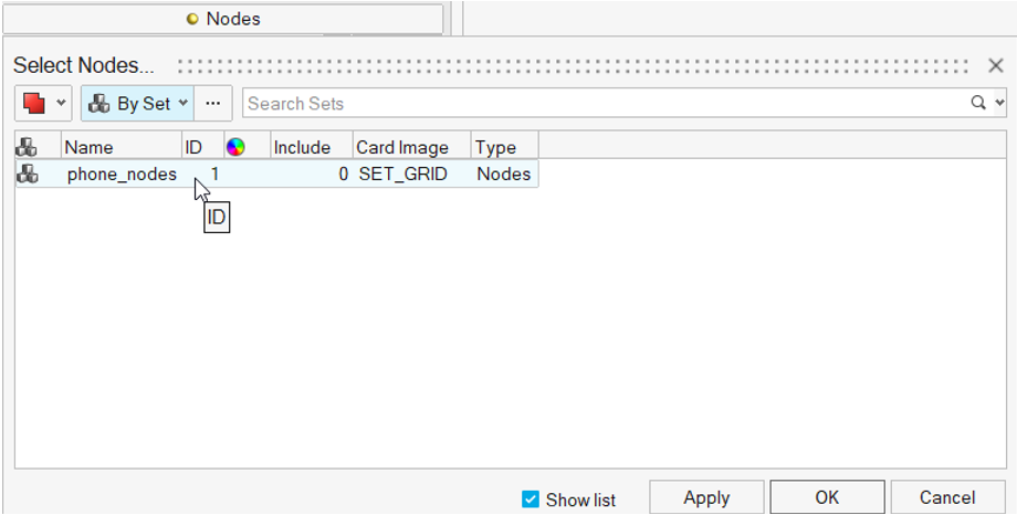
From the list of sets, select phone_nodes.
Figure 11. Phone Nodes Set
Click OK.
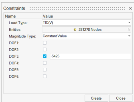
Deselect all DOF check boxes except DOF3.
For DOF3, enter a value -5425.
Figure 12. Definition of Initial Velocity
Click Create.
Click
Close.
Create an Explicit Load Step
In this step, an explicit load step is created referencing the previously defined
load collectors.
In the Model Browser, right-click and select
Create > Load Step.
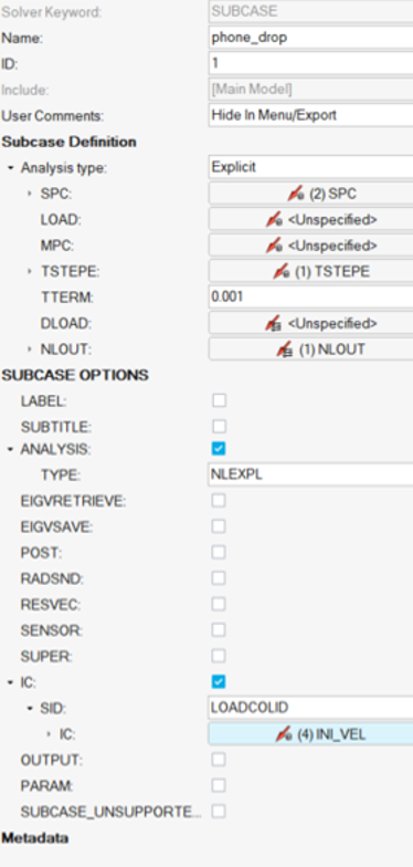
For Name, enter phone_drop.
For Subcase Definition, Analysis type, select
Explicit.
For SPC, click Unspecified > to open Advanced Selection.
Select the SPC load collector and click
OK.
Similarly, for TSTEPE, select the TSTEPE load
collector.
For TTERM, enter 0.001.
For NLOUT, click Unspecified > to open Advanced Selection.
Select the NLOUT Load Step Input and click
OK.
For SUBCASE OPTIONS, select the IC check box.
For IC, click Unspecified > to open Advanced Selection.
Select the INI_VEL load collector and click
OK.
Close the Entity Editor.
Figure 13. Explicit Load Step Definition
Create Control Cards
In this step, control cards for the simulation are defined.
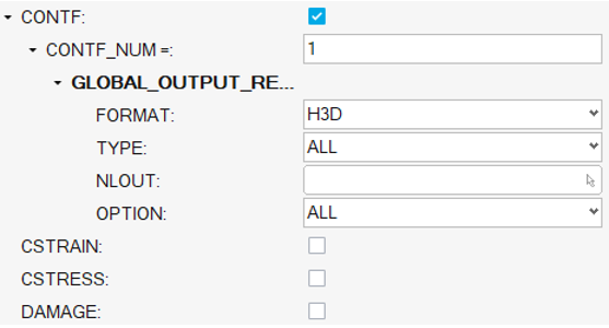
In the Model Browser, right-click and select Create > Cards > Output.
Select the CONTF check box.
For FORMAT, select H3D.
For OPTION, select ALL.
Figure 14. CONTF Settings
Select the DISPLACEMENT check box.
Set FORMAT = H3D and OPTION =
ALL.
Select the STRAIN check box.
Set FORMAT = H3D and OPTION =
ALL.
Select the STRESS check box.
Set FORMAT = H3D and OPTION =
ALL.
Click
Close.
Submit the Job
Run OptiStruct.
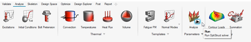
From the Analyze ribbon, click Run OptiStruct
Solver.
Figure 15. Select Run OptiStruct Solver
Select the directory where you want to write the OptiStruct model file.
For File name, enter Drop_test.
The .fem filename extension is the recommended extension
for Bulk Data Format input decks.
Click Save.
Click Export.
For export options, toggle all.
Click Export.
The .fem file is exported. The Compute Console
should open with the file loaded in Input file(s).
In the Altair Compute Console, click
Run.
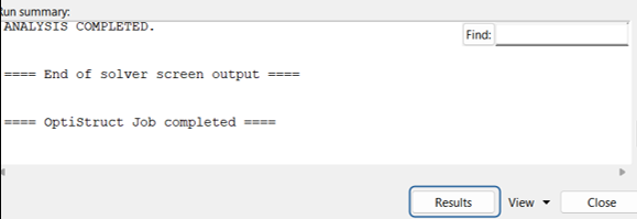
If the job is successful, an "OptiStruct Job Completed" message appears
in the Compute Console Solver View Message Log. New results
files are in the directory where the model file was written. The
Drop_test.out file is a good
place to look for error messages that could help debug the input deck if any
errors are present.
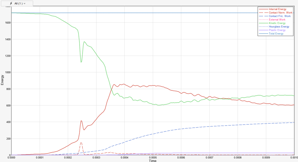
View the Work and Energy Curve Plots
In the Altair Compute Console, click
Results.
Figure 16. Load Results HyperGraph launches and loads the Drop_test
_expl_energy.mvw file, plotting the curves.Figure 17. Work and Energy Curve Plots
View a Contour Plot of Stresses and Displacement
In HyperGraph, select Subcase 1 (phone
drop) to expand the page creation dialog.
Click
to add a page.
Figure 18. Create New Page
On the menu bar, switch from HyperGraph to HyperView.
Click File > Open > Model.
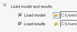
For Load model and results, select the File
icon.
Figure 19. Open Results File in HyperView
Navigate to and select the Drop_test_phone_expl.h3d
file.
Click Open, then Apply.
The results file loads in HyperView.
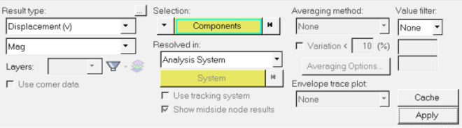
From the ribbon, click Contour.
In the Results tab, select the last time increment at Time =
0.001.
For Results type, select Displacement.
Figure 20. Displacements
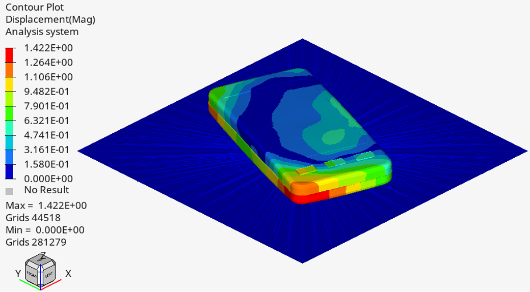
Click Apply.
The contour of the displacement plot is displayed at the final
increment.Figure 21. Displacement Contour

 .
.
 to open Advanced Selection.
 to add a page.
 icon.
icon.