Tutorial Level: Intermediate This tutorial focuses on performing shape optimization on an L-section cantilever beam
modeled with shell elements.
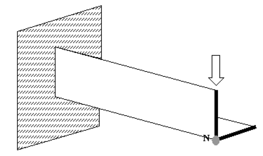
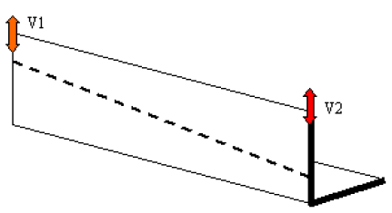
A schematic is shown in . The beam’s design needs to be constrained such
that the vertical deflection at point N should be limited to 2.0mm while minimizing
the amount of material required.Figure 1. Cantilever L-beam Schematic
Before you begin, copy the file(s) used in this tutorial to your
working directory.
The optimization problem for this tutorial is stated as:
Objective
Minimize mass.
Constraints
A given maximum nodal displacement < 2 mm.
Design Variables
Shape of each of the beam flanges.
The following exercises are included:
Set up a shape optimization problem in HyperMesh.
Post-process optimization results in HyperView.
Launch HyperMesh
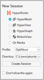
Launch HyperMesh.
In the New Session window, select HyperMesh from the list of tools.
For Profile, select OptiStruct.
Click Create Session.
Figure 2. Create New Session This loads the user profile, including the appropriate template, menus,
and functionalities of HyperMesh relevant for
generating models for OptiStruct.
Open the Model File
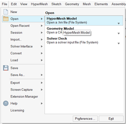
On the menu bar, select File > Open > HyperMesh Model.
Navigate to and select the Lbeamshape.hm file saved in your
working directory.
Click Open.
The Lbeamshape.hm database is loaded into the current
HyperMesh session, replacing any existing
data.Figure 3. Model Import Options
Tip: Alternatively, you can drag and drop the file onto the
viewport from the file browser window.
Set Up the Model
Create Shapes
This section makes use of HyperMorph. For a more detailed
description of the functionality of HyperMorph, refer to
the HyperMorph section of the HyperMesh documentation.
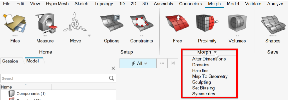
Open the Morph ribbon.
From the ribbon, click the Morph drop-down menu and
select Domains.
Figure 4. Create Domains
In the Domains window, for Type, select Global
Domains.
Click Create.
Similarly, to create local domains, select Type: Local
Domains and click Create.
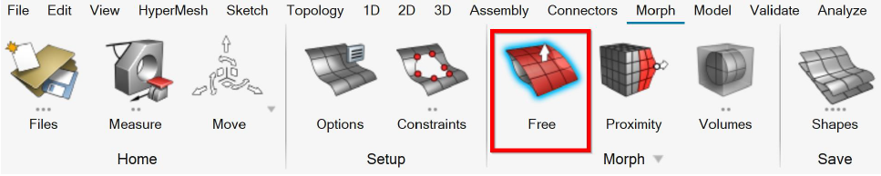
From the Morph ribbon, select Free.
Figure 5. Select Free Tool on Morph Ribbon
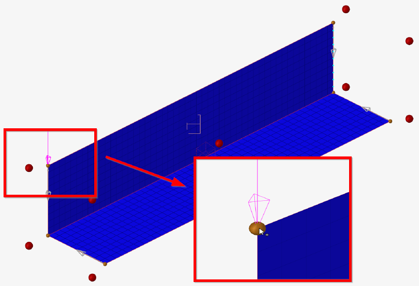
On the guide bar, select Move > Nodes.
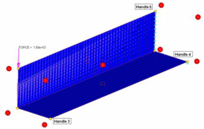
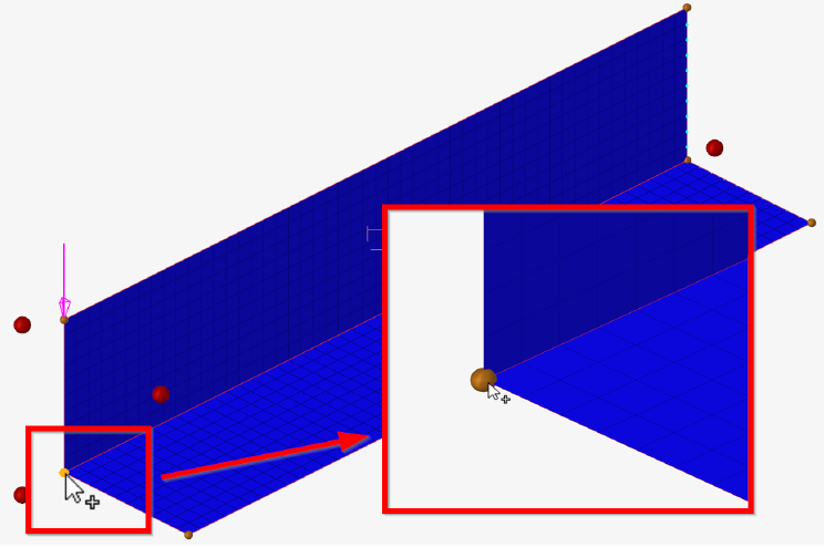
In the modeling window, select the local handle that is
located at the node where the load is applied.
Local handles are indicated by a yellow ball as shown in Figure 6.Figure 6. Select Local Handle
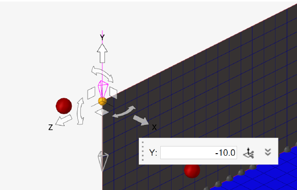
Click the Y-direction arrow and enter -10 in the
microdialog.
Figure 7. Choose Y-direction and Enter -10
Press Enter.
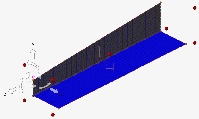
The beam changes shape so that the handle you selected moves -10.0 in the
Y-direction. The mesh is adjusted to this change in shape.Figure 8. Mesh Adjusts to New Shape
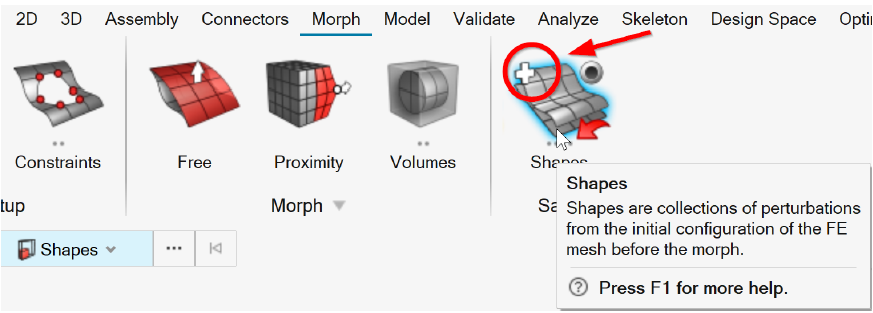
From the Morph ribbon, hover over the Shapes tool and click the
Create (+) satellite icon.
Figure 9. Select Create Shape
The changes made to the original design are saved as
shape1.
Hover over the Shapes tool and click Undo All.
Figure 10. Select Undo All
The model returns to its original shape in the modeling window. This does not undo the created shape; it is
already saved.
Repeat steps 7 through 12 for the local handles 3, 4, and 5 (see Figure 11).
For each local handle, select the Free tool and
then Move > Nodes on the guide bar.
Verify you select the local handles (yellow balls), not the global
handles (red balls).
Tip: To ensure you have selected the right handles, you can
see whether the geometry is morphed in the applied direction of
shape change before you select Undo All.
Translate handles 3 and 4 by x = -10 and handle
5 by y = -10.
Figure 11. Local Handles to be Morphed
Create Design Variables for Shape Optimization
In the Model Browser, double-click on
shapes.
In the Entity Editor, change the last three shape names
to shape2, shape3 and
shape4, respectively.
Select the shape2, shape3, and
shape4 check boxes.
Four shape design variables are created using the shapes that were saved
earlier.Figure 12. Potential Variation of Vertical Flange of L-beam Achieved using the
Described Setup
Create Mass and Static Displacement
In this step, mass and static displacement for nodes is created as responses.
Two responses are defined: a Mass response for the objective function and a
Displacement response for the constraint. A detailed description can be found in the
OptiStruct
User Guide under Responses.
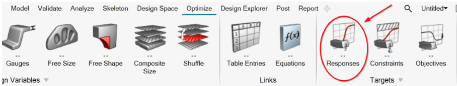
Open the Optimization ribbon and select
Responses.
Figure 13. Select Responses
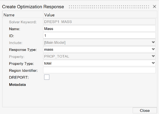
For Name, enter Mass.
For Response type, select mass.
Figure 14. Select Response Type as Mass
Click Close.
A response, mass, is defined for the total mass of the
model.
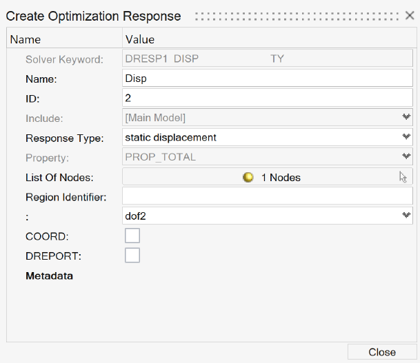
Similarly, create another Response with the name
Disp.
For Response type, select static displacement.
From the list of nodes, select the node with grid ID
84.
This is the free end of the beam.Figure 15. Select Node for Defining Displacement Response
Select dof2.
DOFs 1, 2, and 3 refer to translation in the X, Y, and Z directions.
DOFs 4,
5, and 6 refer to rotation about the X, Y, and Z axes.Figure 16. Create Displacement Response
Click Close.
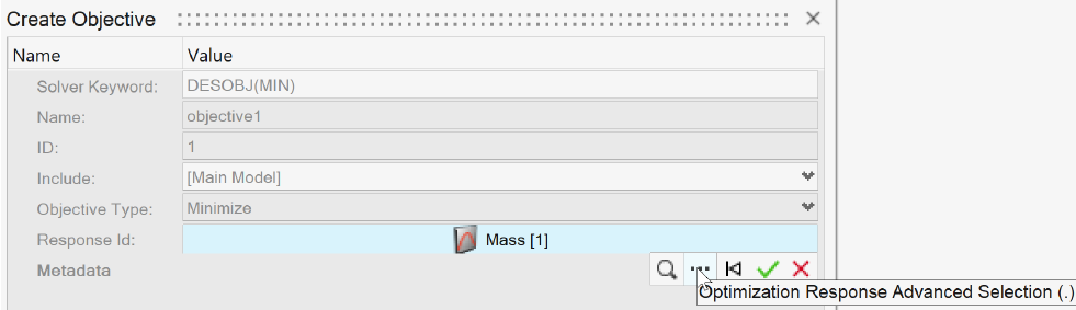
Define Minimize Mass as Objective Function
In this step, the objective is to minimize the mass response defined in the previous
section.
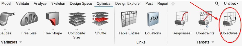
From the Optimize ribbon, select Objectives.
Figure 17. Select Objectives Tool
For Objective type, select minimize.
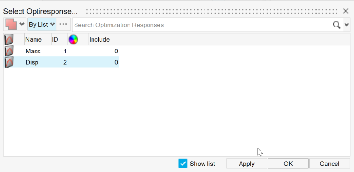
For Response ID, select Unspecified > to open Advanced Selection.
Figure 18. Advanced Selection
In the window, select the Mass response.
Click , then Close.
Apply Design Constraint on Static Displacement Response
A response defined as the objective cannot be constrained (volume, in this case).
A lower bound constraint is defined for the displacement response defined in the
previous section.
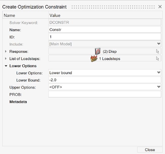
From the Optimize ribbon, select Constraints.
For Name, enter Constr.
For Response ID, select Unspecified > to open Advanced Selection.
From the list of responses, select Disp.
Figure 19. Select Disp Response
Click Apply, then .
For List of loadsteps, open Advanced Selection and
select load.
Click Apply, then .
For Lower options, select Lower bound and enter
-2.0.
This is a lower bound as the response is negative.Figure 20. Constraint Window with all Selections
Click Close.
A constraint is defined on the response Disp. The constraint is a lower
bound with a value of -2.0. The constraint applies to the subcase
Load.
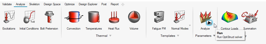
Submit the Job
Run OptiStruct.
From the Analyze ribbon, click Run OptiStruct
Solver.
Figure 21. Select Run OptiStruct Solver
Select the directory where you want to write the OptiStruct model file.
For File name, enter Lbeamshape_opt.
The .fem filename extension is the recommended extension
for Bulk Data Format input decks.
Click Save.
Click Export.
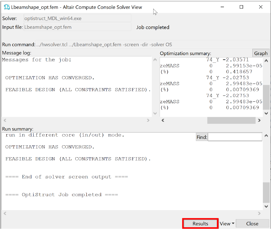
In the Altair Compute Console, click
Run.
If the job is successful, an "OptiStruct Job Completed" message appears
in the Compute Console Solver View Message Log. New results
files are in the directory where the model file was written. The
Lbeamshape_opt.out file is a good
place to look for error messages that could help debug the input deck if any
errors are present.
Figure 22. Run Summary
Post-process the Results
Shape contour information is output from OptiStruct for all iterations. In addition, displacement and
stress results are output for the first and last iterations by default. This section
describes how to view those results in HyperView.
View Deformed Structure
It is helpful to view the deformed shape of a model to determine if the boundary
conditions have been defined correctly and also to check if the model is deforming
as expected. In this section, review the deformed shape for the last design
iteration and a scale factor, and overlay the undeformed shape.
Open the results file Lbeamshape.h3d in HyperView.
From OptiStruct, you can launch HyperView by selecting Apps > HyperView and choosing the .h3d file. Alternatively,
you can open the file from the Altair Compute
Console by clicking Results.
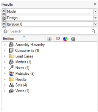
From the drop-down menu, select the last iteration, Iteration
8.
Figure 23. Select Last Iteration
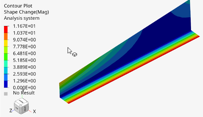
Click Contour.
Figure 24.
For Result type, select Shape change (v).
Click Apply.
The final shape for Iteration 8 is plotted.Figure 25. Final Shape
View a Transient Animation of Shape Contour Changes
To start the animation, click Play.
The seek slider and playback speed slider (top and bottom respectively) are
located next to the playback controls.Figure 26. Animation Play Button and Slider
Use the slider to adjust playback speed and skip between frames of the
animation.
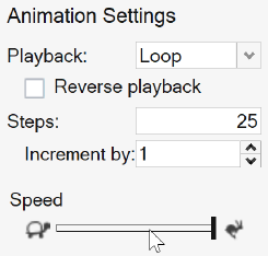
Click Advanced options for more playback options such as:
Increase or decrease speed
Select playback type
Change the number of increments
Figure 27. Advanced Options for Animation Settings
Plot a Contour of Displacements
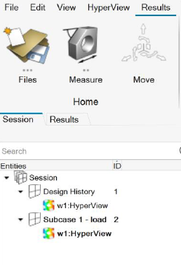
On the Model Browser, open the
Session tabl.
Figure 28. Session Tab
Double-click Subcase 1 - load 2.
Click Contour.
Figure 29.
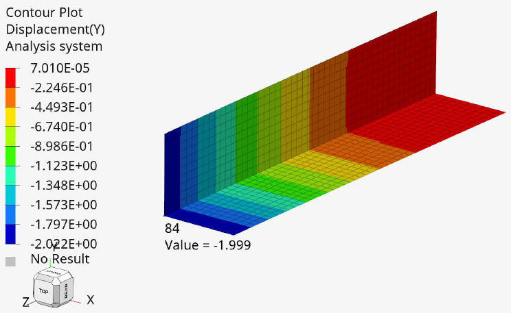
For Result type, select Displacement (v).
Select the Y component of the Displacement, as this was the chosen design
constraint.
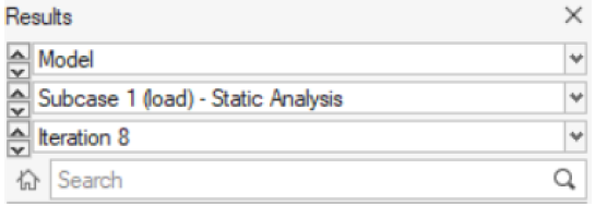
From the drop-down menu, select the last iteration, Iteration
8.
Figure 30. Choose Subcase and Last Iteration
Click Apply.
A plot of the displacements on the final shape is displayed. The maximum
displacement in Y for the last Iteration is still below 2.0 at Node 84, which
was the chosen design constraint.Figure 31. Contour of Displacement in Y


 to open Advanced Selection.
 , then Close.

 Play.
The seek slider and playback speed slider (top and bottom respectively) are located next to the playback controls.
Play.
The seek slider and playback speed slider (top and bottom respectively) are located next to the playback controls.
 Advanced options for more playback options such as: