
MV-9000: Bouncing Ball Tutorial
In this tutorial, you will learn how to model a simple 1 DOF mechanism using the Msolve Python API.
If you are running this tutorial as IPython notebook, you can interactively execute each code cell by clicking SHIFT-ENTER. The output of the Python code (if any) is displayed and the execution jumps to the next cell.
Load the Msolve Module
In [2]: from msolve import*Create a Model
To create the pendulum mechanism, you must first create a model.
In [3]: model = Model() Add Units and Gravity
After creating a model, you can add details, units, and other entities such as gravity and ground. Most entities have default properties. For example, when you create the solver unit set without specifying arguments, you are essentially creating SI units.
-
Issue this command:
In [4]: units = Units() #SI -
Similarly, you can create the gravitational acceleration field.
In [5]: grav = 9.807 gravity = Accgrav(igrav=0, jgrav=0, kgrav=-grav) -
You can now create the ground part by using the Part class and specifying the
ground Boolean attribute as 'True':
In [6]: ground = Part(ground=True)
Create Markers
Next, you can create markers on the ground part. A marker is defined by a geometric point in space and a set of three mutually perpendicular coordinate axes emanating from that point. It can be used as a reference frame of the part that it belongs to.
In [7]: global_ref = Marker(part=ground) Create a Geometry Object
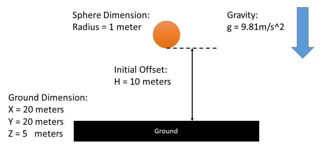
For animation purposes, you can create a geometry object. In this case, a box representing the ground. According to the documentation, a box requires a center marker and its x,y,z dimension.
-
Issue this command:
In [8]: box=Box(cm=global_ref, x=20, y=20, z=5)You can similarly create the ball by first creating a part with mass and then creating a sphere located at the cm (center of mass) of the part. Inform the solver of the mass and cm of the part unless you are creating a ground part.
The mass of the sphere is given by:
m=V×ρ=43πr3×ρThe inertia property is given by:
Ixx=Iyy=Izz=2mr25 -
Issue the command:
In [9]: # define the cm of sphere
radius = 1
initial_offset = 10
p = Point(0,0,radius+box.z/2.0+initial_offset)

# calculate the mass and inertial property of sphere
volume = (4.0/3.0)*radius**3
density = 1522
mass = volume * density
ixx = iyy = izz = 2.0 * mass * radius ** 2 / 5.0

# create part and cm for the sphere
sphere= Part(mass = mass, ip = (ixx, iyy, izz, 0, 0, 0 ), qg=p)
sphere.cm = Marker(body=sphere)

# create the geometry
geo = Sphere(cm=sphere.cm, radius = radius)
Define the Contact Force
You can define the contact force between the ground and the sphere. First, define a marker on each part at the contacting point. These two markers are used in the force calculation and displacement monitor.
-
Issue this command:
In [10]: marker_i = Marker(part = sphere, qp = (0,0,-radius), xp = (1,0,0), zp = (0,0,100)) marker_j = Marker(part = ground, qp = (0,0,box.z/2.0), xp = (1,0,0), zp = (0,0,box.z/2.0+1)) -
Call Sforce to calculate the contact force as the ball
moves. The input function should be a MotionSolve
expression and the z axis of marker j defines the direction that the force
applies.
In [11]: input_function =
"IMPACT(DZ({I}, {J}, {J}),VZ({I}, {J}, {J}),{G},{K},{E},{C},{D})"
.
format( I=marker_i.id,J=marker_j.id, K=5e9, G=0.00, E=1.0, C=0.8e5, D=0.0 )
contact_force = Sforce(i = marker_i.id, j = marker_j.id,
type=
"TRANSLATION"
, function = input_function)
Add Joints and Requests
You can add a translational joint here to prevent the ball from flapping around (although it is not necessary). To create a joint, define the type of the joint as well as the markers that the joint is placed on. The z axis of marker j defines the direction of translational joint.
You can also create a request. Requests define output channels in MotionSolve and are written to MotionSolve output files so that they may be used for plotting and signal processing by HyperGraph. Requests can be defined using runtime expressions, built-in functions (MOTION, FORCE, FIELD, and so on), or user-written functions.
-
Create a displacement request using the predefined "DZ" method and then create
another request to track the contact force:
In [12]: # Translational Joint, prevent the sphere flapping around joint = Joint (type="TRANSLATIONAL",i=marker_i.id,j=marker_j.id) # Adding monitor into the model model.forceRequest = forceRequest = Request(f2="FZ({I},{J},{J})".format(I=marker_i.id, J=marker_j.id)) model.dispRequest = dispRequest = Request(f2="DZ({I}, {J}, {J})".format(I=marker_i.id, J=marker_j.id)) -
Call Sforce to calculate the contact force as the ball
moves. The input function should be a MotionSolve
expression and the z axis of marker j defines the direction that the force
applies.
In [13]: input_function =
"IMPACT(DZ({I}, {J}, {J}),VZ({I}, {J}, {J}),{G},{K},{E},{C},{D})"
.
format( I=marker_i.id,J=marker_j.id, K=5e9, G=0.00, E=1.0, C=0.8e5, D=0.0 )
contact_force = Sforce(i = marker_i.id, j = marker_j.id,
type=
"TRANSLATION"
, function = input_function)
Run the Simulation
At this point you are ready to run a transient analysis. The simulate method is invoked on the MBS model. A validation process is performed on each of the entities that make up the model. This is a necessary step to ensure that only correct models are being simulated. Note that the simulate command can be invoked with an optional flag, returnResults, set to True. This stores the results of the simulation into a run container for further post-processing, as shown below.
-
Issue the following command:
In [14]: run=model.simulate(type="DYNAMIC", returnResults=True, end=50, steps = 10000) -
In the following example, you are extracting the
model.despRequest from the run container. The purpose is
to have a convenient data structure for extracting time varying results.
In [15]: dz=run.getObject(model.dispRequest) -
Use the dz object to plot the displacement along the global z axis, using the
matplotlib module available in IPython notebook. The plot is displayed inline.
You can see how the magnitude of bouncing changes as time goes.
In [16]: %matplotlibinline
frommatplotlibimport pyplot
pyplot.plot(dz.times, dz.getComponent(1))
pyplot.xlabel('Time(s)')
pyplot.ylabel('Displacement(m)')
pyplot.show()
Figure 2. The bouncing magnitude decreases each time the ball hits the ground because a damping exists in the definition of contact force.