Green House Noise - Result Generation Tab
Define Green House Panels
- Vehicle Type
- Select from the following options:
- Sedan
- Hatch Back
- Crossover
- Two Row Seat SUV
- MPV
- Three Row Seat SUV
- Active Panels
- Select the panel(s) to be included in the green house noise analysis. The panel's material and geometry parameters can also be updated.
- Click the Filter icon,
 ,
to display the Filter Panel dialog. Use this dialog to change the
panel's status.
,
to display the Filter Panel dialog. Use this dialog to change the
panel's status. - 18 panels are supported for each vehicle type.
Figure 2. 
Figure 3. 
- Apply Symmetry
- Select this option to ensure the passenger side's glass material, geometry, and loads are the same as the driver's side.
- Lamination
- Select Yes if the panel is laminated.
Figure 4. 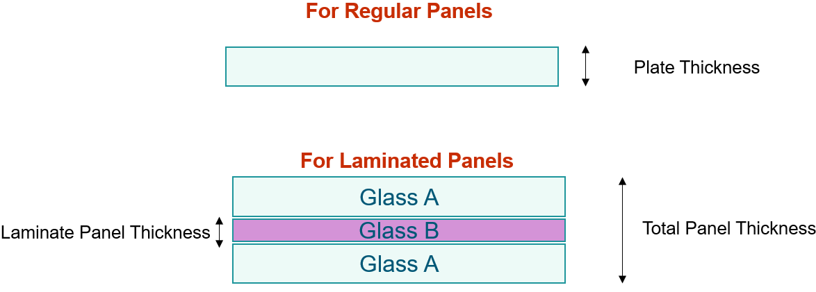
- Materials
- Click Material Database to create and maintain the material properties as a database on a local or remote machine.
- Materials are defined as IsoElastic or ViscoElastic for glass and
laminate materials, respectively. You can add and delete materials as
necessary.
Figure 5. 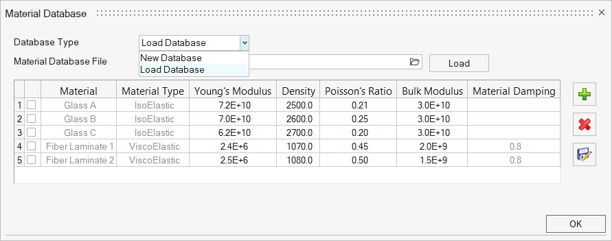
- Damping
- Create damping properties for each panel as a database.
- Damping is defined as structural or acoustic for cabin reverberation and
panel materials, respectively.
Figure 6. 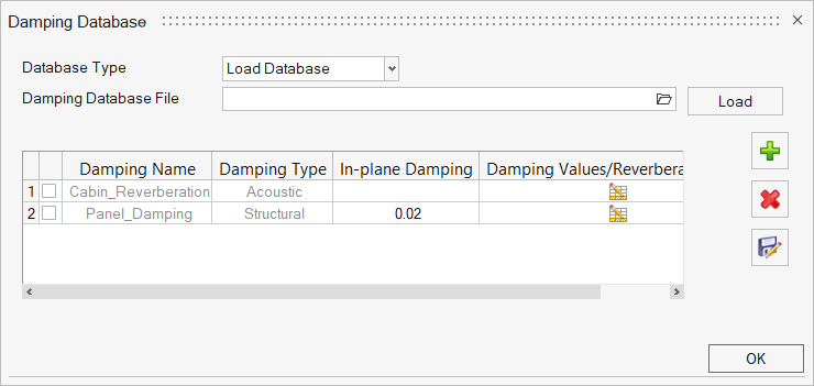
- Signal Processing Parameters
- From the Element Analysis tab, click Signal Processing Parameters to convert the transient data to frequency domain data (narrow band and broadband).
-
Figure 7. 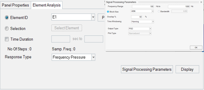
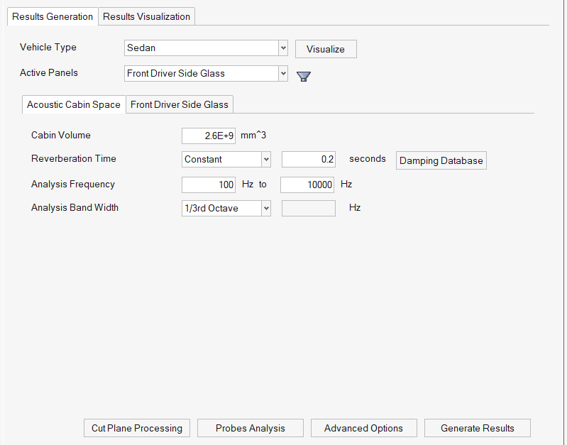
- Acoustic Cabin Space
- Use the Acoustic Cabin Space tab to specify the
acoustic cabin space volume, reverberation time, analysis frequency
range, and analysis bandwidth of the output interior noise curves.
Figure 8. 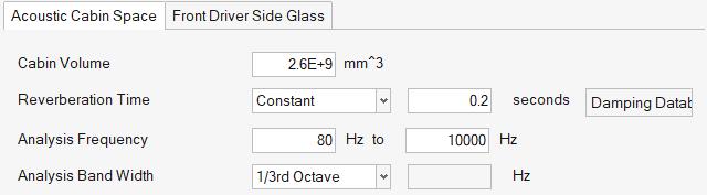
- Probes Analysis
- Use Probes Analysis to post-process the probes
pressure results obtained from ultraFluidX.
- Use probes or surface pressure transient result files as input for probes analysis.
- Both frequency spectrum and transient signal plots can be displayed.
- The time-domain signal is multiplied with the cp to pressure factor.
- Options for the output type for the frequency domain can be PSD or SPL. You can generate a narrowband or octave band plot.
- Use the individual or the surface averaged response of elements for processing.
Figure 9. 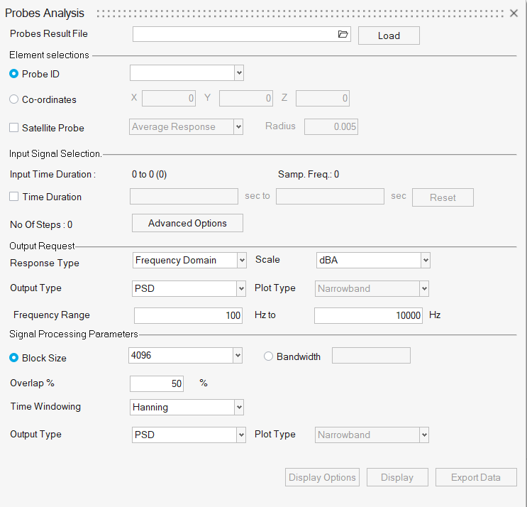
- Cut Plane Processing
- Use Cut Plane Processing to generate dBMap and frequency filtered
transient animation.
Figure 10. 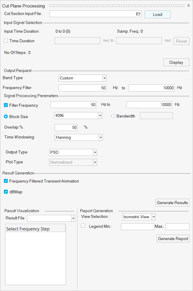
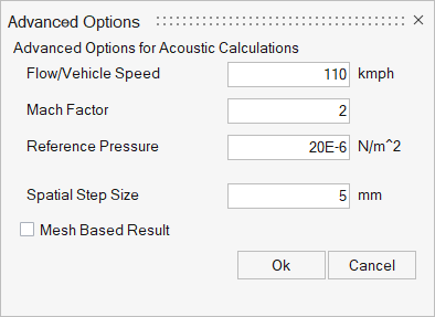
- Advanced Options
- From the Advanced Option panel, you can set the parameters required for
acoustic dBMap and contribution calculations.
Figure 11.