HL-T: 1090 Random Fatigue Analysis Using FRF Stresses and Power Spectral Density of Loading Versus Frequency (Input PSD)
Tutorial Level: Beginner
In this tutorial you will:
- Import a model to HyperLife
- Check that the FE result file contains a frequency response function (FRF) subcase with element stresses
- Select the SN module with a Random (Input PSD with FRF) loading type and define its required parameters
- Create and assign a material
- Create a random fatigue event with Input PSDs
- Evaluate and view results
Before you begin, copy the file(s) used in this tutorial to your
working directory.
Import the Model
-
From the Home tools, Files tool group, click the Open Model tool.
Figure 1. 
-
From the Load model and result dialog, browse and select
HL-1090\Antenna_Vibration_Fatigue.h3d for the model
file.
The Load Result field is automatically populated. For this tutorial, the same file is used for both the model and the result.
-
Click Apply.
Figure 2. 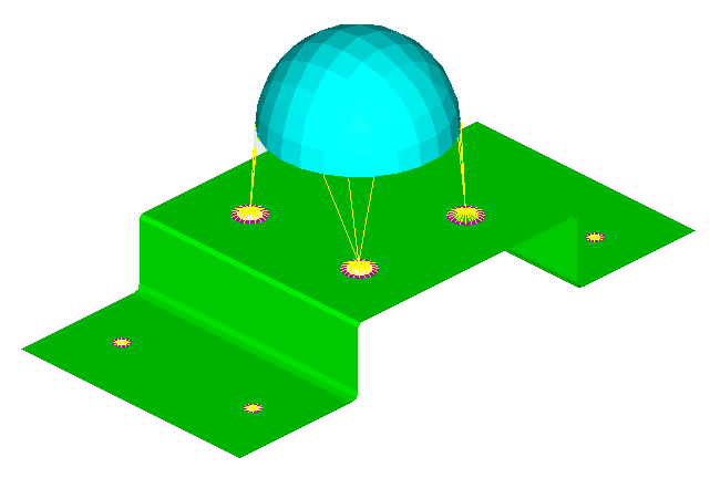
Tip: Quickly import the model by dragging and
dropping the .h3d file from
a windows browser into the HyperLife
modeling window.
Check That the FE Result File Contains a Frequency Response Function Subcases with Element Stresses
-
From the Results Browser, click the second drop-down menu
and select Subcase 1 (Load_X).
If the Results Browser is not open, click from the menu bar.
Figure 3. 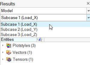
-
From the View Controls toolbar, click
 .
The Contour panel opens.
.
The Contour panel opens. - From the panel area, select Element Stresses (2D & 3D) (t) (c) from the first Result type drop-down menu.
-
Select XX from the second Result type drop-down
menu.
Figure 4. 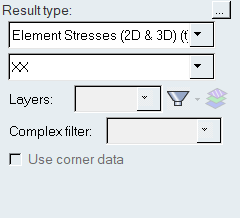
-
Click Apply.
The model is contoured.
- Observe the element stress plot in the modeling window.
- Select Subcase 2 (Load_Y) from the second drop-down in the Results Browser.
- Observe the updated element stress plot in the modeling window then select Clear Contour in the panel area.
- Exit the Contour panel.
Define the Fatigue Module
-
Click the SN tool.
The SN tool should be the default fatigue module selected. If it is not, click the arrow next to the fatigue module icon to display a list of available options.
Figure 5. 
The SN dialog opens. -
Define the SN configuration parameters.
Figure 6. 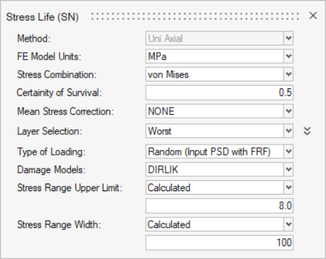
- Exit the dialog.
Assign Materials
-
Click the Material tool.
Figure 7. 
The Assign Material dialog opens. - Activate the checkbox next to Plate.
-
Select a material.
- Click the Material DB tab.
- In the Search field, enter 189 and press Enter.
- From the search results, right-click Steel 1005, HR Sheet, Su = 359.0(189) and select Add to Assign Material List from the context menu.
-
Return to the Assign Material Data tab. Using the
Material drop-down menu, select Steel 1005, HR Sheet, Su =
359.0(189) for Plate.
The Material list is populated with the materials selected from Material Database and My Material.
Figure 8. 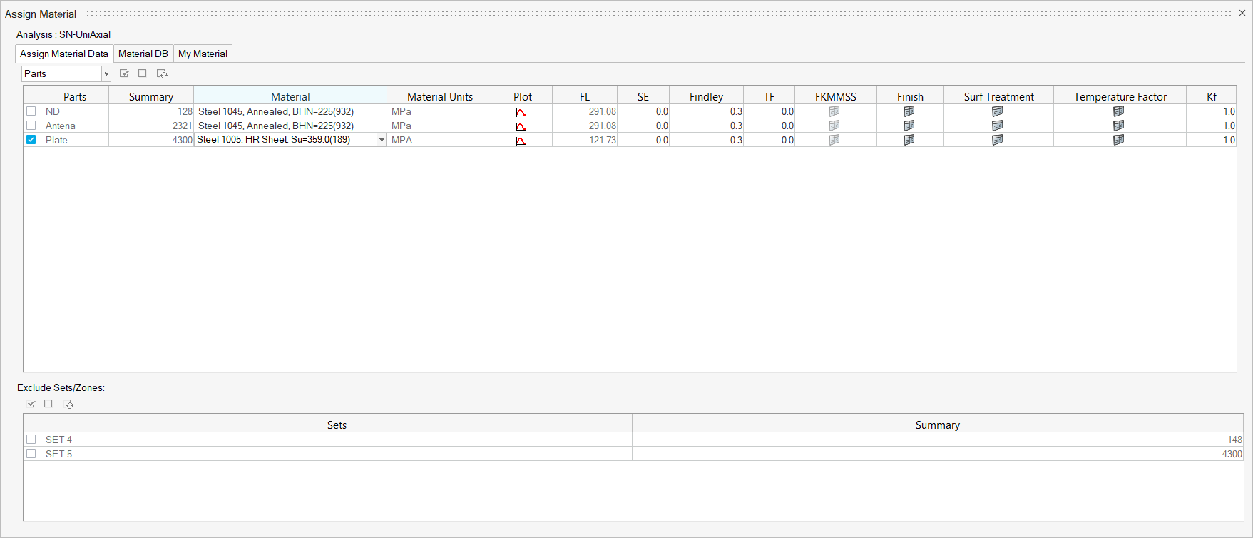
- Exit the dialog.
Create a Random Response Event
-
Click the Load Map tool.
Figure 9. 
The Load Map dialog opens. - From the Channel Type drop-down menu at the top of the dialog, select Input PSD: Real & Imaginary.
-
Load PSD vs Frequency data (input PSD that is to scale the FRF stresses).
-
Click
 in the Choose File
field and browse for psd_X.csv,
psd_Y.csv, and
psd_Z.csv.
in the Choose File
field and browse for psd_X.csv,
psd_Y.csv, and
psd_Z.csv.
-
Click
 to add the load case.
-
Click
- Optional:
Click
 to view a plot of the loads.
- Select Subcase 1 (Load_X), Subcase 2 (Load_Y), and Subcase 3 (Load_Z).
-
On the bottom half of the dialog, click to create an Event_1
header.
The possible correlations of Subcase 1, Subcase 2, and Subcase 3 are listed under the event.
-
Select the three psd files and drag-and-drop them into the
Event header.
Note: Any blank correlations are not considered in the calculation.The following pairs are created:
- Subcase 1 with psd_X
- Subcase 2 with psd_Y
- Subcase 3 with psd_Z
- Activate the Event_1 checkbox.
-
Set the Exposure Time for the event to 18000.
Figure 10. 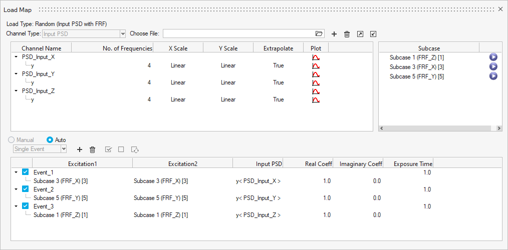
- Exit the dialog.
Note: If Mean Stress correction is to be applied, a static subcase, if present in the
result file, will be listed in the Subcase window and can be drag and dropped onto
the event (no channel is required to be paired).
Evaluate and View Results
-
From the Evaluate tool group, click the
Run Analysis tool.
Figure 11. 
The Evaluate dialog opens. - Optional:
Enter a name for the run.
Figure 12. 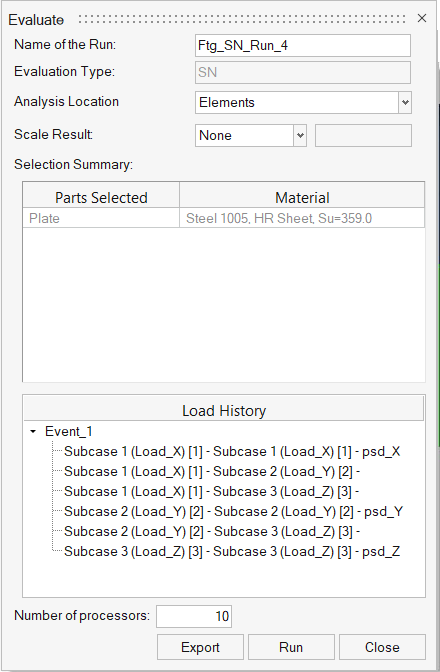
-
Click Run.
Result files are saved to the home directory and the Run Status dialog opens.
- Once the run is complete, click View Current Results.
-
Use the Results Explorer to
visualize various types of results.
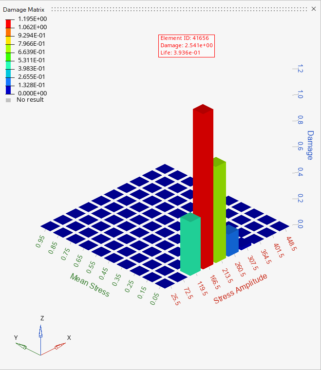
Figure 13. 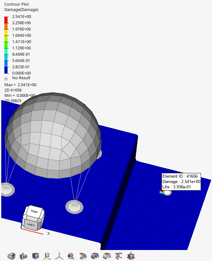
Figure 14.