
HMCFD-T: 0001 Introduction to HyperMesh CFD User Interface
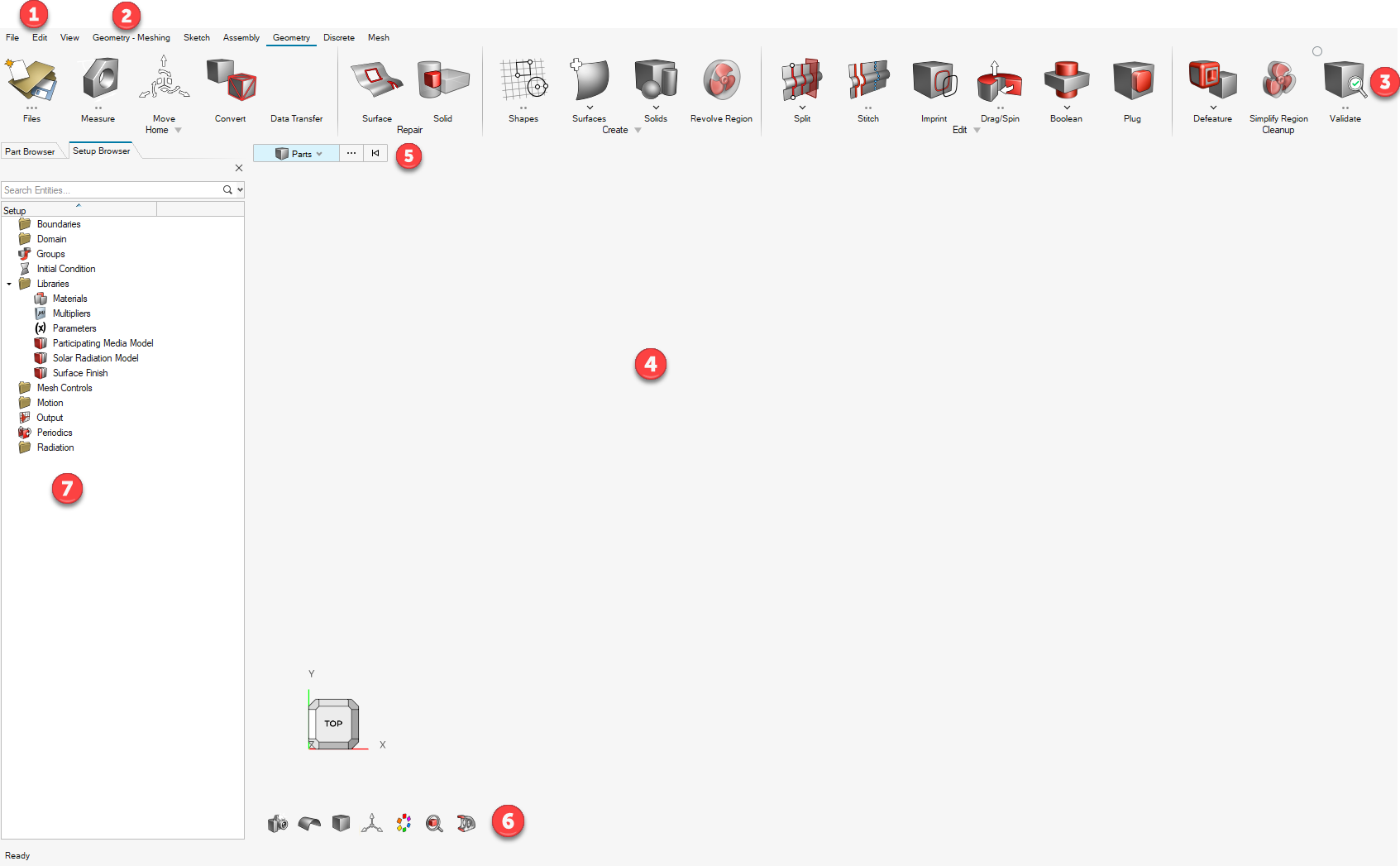
The HyperMesh CFD graphical user interface can be divided into seven general categories as shown in the figure above.
- The menu bar contains the drop-down menus for File input-output, Edit, and View operations.
- The modeling environment switcher is used to populate relevant ribbons and tools based on modeling tasks.
- Ribbons contain various functionalities and tools available in HM-CFD. Navigate
between various ribbons by clicking the ribbon tabs to the right of the modeling
environment switcher. After selecting a ribbon, the corresponding tool icons are
displayed on the screen. The functionalities of various ribbons and corresponding
tools are briefly explained in this section.
- Sketch ribbon
- The Sketch ribbon provides multiple ways to define sketching plane
by selecting planes aligned with global coordinate systems. You can
also get references of existing geometry by cutting geometry or
projecting geometry to a plane. It provides capabilities to create
sketches using multiple interactive tools. A dimensioning capability
enables you to parametrize dimensions of sketches. One of big use
case for CFD is to get cutting lines of rotating geometry and create
a non–cylindrical axisymmetric MRF region around them.
Figure 2. 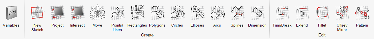
- Geometry ribbon
-
The Geometry ribbon consists of tools for repairing, creating, editing, and validating the geometry.
When a geometry file is imported, the Repair tools can be used to detect any defects present in the CAD model like intersections, free edges, duplicates, sliver surfaces, and so on and fix those errors.
The tools available under the Create sub-section can be used to create geometric entities like points, lines, surfaces, and solids.
The tools required for performing operations like plugging cavities, stitching surfaces, and so on are available under the Edit sub-section.
The Defeature tool can be used to resolve defects or model a new geometry, while the Validate tool can be used to detect any defects present in the CAD model. This process is usually known as CAD cleanup.
Figure 3. 
- Discrete ribbon
-
The Discrete ribbon consists of tools used for working with FE geometry. You can cap openings, connect geometry, define local or proximity-based wrap controls, enclose the model, remesh the enclosed results, and fix the mesh quality.
-
Figure 4. 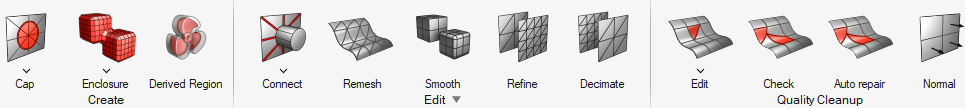
- Assembly ribbon
- The Assembly ribbon is useful for finding, managing, and organizing the parts in your model.
-
Figure 5. 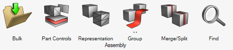
- Flow ribbon
-
The Flow ribbon contains tools for setting up simulation parameters, solver settings, and reference properties such as material properties, heat sources, porous media, and so on. The Setup sub-section is where you set up the physics equations and solver settings as well as create material models, multiplier functions, and parameters.
Figure 6. 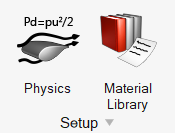
The Domain sub-section contains tools for assigning reference properties such as materials, heat and momentum sources, and reference frames to volumes.Figure 7. 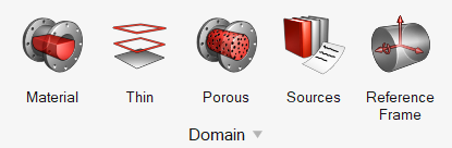
Surface boundary conditions such as inlets, outlets, and far fields, can be assigned using the tools under the Boundaries sub-section. By default, all the surfaces are assigned a boundary condition of type ‘auto_wall’ and are placed under Default wall. Refer to the AcuSolve Surface Processing manual for more information about auto_wall. As you assign boundary conditions to the surfaces, they are moved into the respective group.Figure 8. 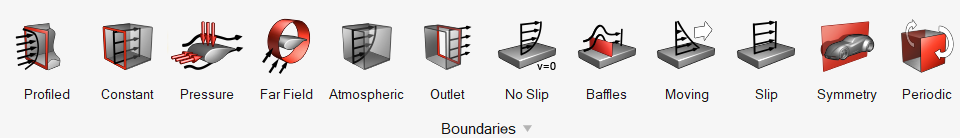
- Radiation ribbon
-
The Radiation ribbon is where you define radiation physics, create thermal, solar, and participating media models, and apply radiation parameters.
Figure 9. 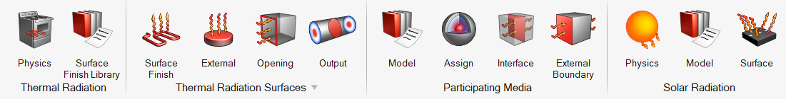
- Motion ribbon
-
Mesh boundary conditions and mesh-motion-related parameters can be defined using the tools available in the Motion ribbon. Parameters such as mesh motion type and mesh displacement constraints can be defined here. In addition to the mesh boundary conditions, code coupling with external codes such as OptiStruct and MotionSolve can be defined here.
Figure 10. 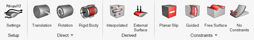
- AcuTrace ribbon
- The AcuTrace ribbon computes particle
traces as a series of segments solving particle motion. It computes
traces for unsteady as well as steady flow fields, for flows with
mesh motion as well as without, and for flows computed on meshes
with interface surfaces. To solve a problem with AcuTrace, you must first run AcuSolve. You can set up for finite mass and
massless particles.
Figure 11. 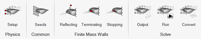
- Mesh ribbon
-
Meshing parameters such as surface mesh controls, boundary layer parameters, volume mesh parameters, and zone meshing parameters can be defined here. This ribbon also has tools for local remeshing. Once all the mesh controls are defined, you can generate the mesh using the Volume tool.
Figure 12. 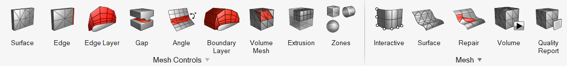
- Aerodynamics and Aeroacoustics Setup
- The setup ribbon is used carry out external aerodynamics and fan
noise simulations with the ultraFluidX
solver.
Figure 13. 
- Solution ribbon
-
The Solution ribbon is used to set up monitors for any individual point, surface, or volume set output. The Field tool is used to set the nodal output frequency for the entire model. The Initialize tools are used to set the nodal initial conditions for variables like pressure, velocity, and variables specific to each turbulence model.
Figure 14. 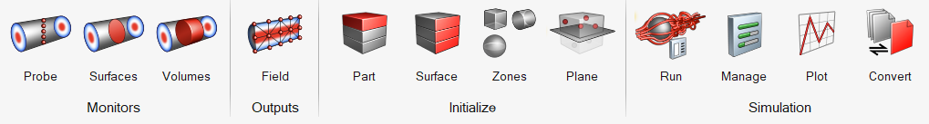
Once the complete set up is done, the Run tool is used to launch AcuSolve. Once the AcuSolve run parameters are set, the simulation can be started, and you can monitor the status of the run using the run manager.
- Post ribbon
- The Post ribbon is where you can post-process the results. The
Visualize tools under the Post ribbon can be used to create things
like plots, streamlines, iso surfaces, and section cuts. The
Measures tools can be used to probe variables at desired
locations.
Figure 15. 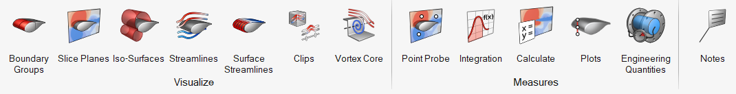
- Morphing Ribbon
- The Morphing ribbon is used to morph mesh or FE geometry. You can define constraints to fix some nodes or define relative movement.
- Once morphing is done, you can create shapes and design variables
using the “Shape” tool and submit DOE studies using “DOE Study”
tool.
Figure 16. 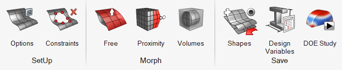
- The modeling window is where the model is displayed. The
model display can be manipulated using the view controls shown in the table below.
Clicking on the model will highlight the entity being selected and right-clicking on
an entity will give you additional options for the operations that can be done based
on the context. Some of the functions available using right-click are Show, Hide,
Isolate, Select, Advanced select, Create groups, and so on.
Button Operation Middle mouse scroll Zoom in and out Right-click hold and drag Pan the model Middle mouse click hold and drag Rotate the model Left-click Select entity Ctrl + Left-click Select multiple entities Left-click hold and drag Window select Shift + Left-click Deselect entities - The entity selector enables you to control what entities can
be selected using the left-mouse button. The selector can be set to any of the
entities shown in the figure below. When you open any tool, the selector is
automatically set to the entity (entities) which are appropriate for that
command.
Figure 17. 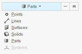
- The visualization of the model can be controlled using the tools available in View
Controls toolbar. The display of mesh, model coloring, section cuts, standard views,
and so on can be controlled using these tools.
Figure 18. 
- The browsers show the entities and setup parameters in the model and list them in a tree structure. They can be turned on or off from the View menu. Some common functions that can be performed in all browsers are show, hide, and isolate.