Altair HyperMesh CFD 2023 Release Notes
Highlights
HyperMesh CFD 2023 introduces a new solution-centric streamlined user interface which provides end-to-end workflows for aerodynamics, aeroacoustics, internal flow, multiphase flow, thermal and moving mesh simulations. A modern UI layout with intuitive workflows provides fast and robust tools for geometric modeling, case setup, post-processing, and design exploration, enabling you to carry out large complex simulations efficiently.
- Seamless end-to-end workflow for aerodynamic and fan noise simulations.
- Improved data management between discrete geometry and aerodynamics setup environments.
- Lite modeling environment
- Volume refinement zone creation utility
- Revolve region tool to create MRF regions automatically
- CAD Wrapper improvements
- Auto seal for CAD Wrapper
- Local control support
- Performance improvement
- Robustness to get clean wrap mesh
- Template manager improvements
- Model organization improvements
- Graphics performance improvements for FE geometry models
- Adaptive two-way wall model
- Enhancements to the fan guide panel workflow
- Accelerated import of parts from pre-processor using thread parallelization
- Python API to run a uFX simulation
- Volume rendering added to part display properties
- Measures: General Signal Processing (GSP) workflow for wind noise calculations
- Engineering Calculator: Calculate uniformity index on a surface, slice plane or iso-surface
- Vortex core: Threshold the vortex core based on vorticity magnitude or vortex core line length
- Import STL files for geometry viewing
- Additional colormap options are available for automatic report generation
- Morphing environment
- Morphing tools
- Tool for DOE studies and process automation
General
New Features
- Ribbon Hints
- Ribbon hints have been added to help identify tools that have multiple
pick targets or open a secondary ribbon. They are small indicators that
appear in the ribbon between a tool’s icon and label. The number of dots
represents the number of pick targets in a tool, including some that are
hidden until hovering over the tool.
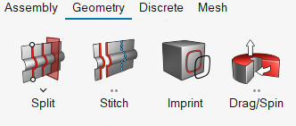
Figure 1.
Known Issues
- On certain machines, when the Enter and Backspace keys are used one after the other while renaming or searching in the Part Browser, a rectangular symbol is shown in the edit field in which you are typing.
Solution Layers
New Features
- Seamless end-to-end workflow for aerodynamic and fan noise simulations
- A new UI layer to enable solution-centric workflows. You are able to carry out end-to-end workflows by traversing through modeling environments available in the UI. There are 3 major aspects of this UI layer:
- Improved data management
- You can work on different modeling environments, and data management of all modeling environments or data transfer between environments is taken care of by the workflow. All data from different environments is packaged in a single file, and on opening the file data is passed to the relevant modeling environment.
Geometric Modeling
New Features
- Lite modeling
- Added a new way to load lite representation of CAD geometry. It affects the following workflows:
- Volume refinement zone creation utility
- A new tool “Derived Region” is added to create volume refinement zones
and projected mesh. You can create the following regions using this
tool:
Enclosed region: Enables you to create refinement zones enclosing selected parts with specified offset distance.
Offset region: Enables you to create refinement zones by offsetting selected parts with specified offset distance.
Projected region: Creates a mesh by projecting inputs on specified direction. Useful for calculating frontal area.
- Revolve region
- A new tool to create an MRF region automatically around a selected solid part is added. You can specify offset distance. You have the option to get the revolved solid as output or a spin surface. With the “Spin Surface” option, you can edit/simplify the surface and then revolve it manually.
Enhancements
- CAD Wrapper improvements
- CAD Wrapper has significant improvements in terms of new features, robustness and performance. The following are major or improvements:
- Template manager improvements
- The template manager has gone through a lot of new improvements:
- Supports part name-based, part metadata-based grouping
- New operations: “Bulk Operation”, “Auto cleanup” and “Volume refinement” added which help to automate aerodynamic modeling.
- Model organization improvements
- Added a new option in the right-click menu to organize elements to any parts. Also added capability to split mesh parts based on connectivity which helps to split models which come as a single part.
- Graphics performance improvement for FE geometry model
- FE Geometry data type rendering performance is improved significantly to make rendering options like show/hide/isolate, selection - deselection instant. Operation performance is improved as well.
Case Setup
New Features
- Adaptive two-way wall model
- A new “adaptive two-way” wall model coupling is introduced which replaces the old “two-way” wall model coupling as the default.
Enhancements
- Fan Guide Panel
- The fan cylinder dimensions are more robust to changes.
- For larger models where computing the volume takes time, a busy cursor is displayed to inform you.
- Overset cylinder volume is centered on adjusting the height.
- Solid revolution volume creation is retried with multiple tolerances for enhanced robustness.
- Python API
- New API has been created to help you set up a simulation and run the solver in the same script. You can invoke vwt.RunUfx(runDir) from the Python window to run the simulation on a Linux machine with a compatible GPU.
- Units Import Dialog
- The import dialog for unit selection has been updated to allow you to interact with the model before choosing the units.
Resolved Issues
- XML import/export errors have been fixed for:
- Fan template with overset volume
- Section cuts
- Fan cylinder volume dimensions requested by user are respected. Additional padding is no longer applied.
- Fan refinement element size is updated consistently.
- Undo/Redo works correctly for fans with Overset/MRF volumes.
- Units import in mm does not affect material properties.
- Section cut visibility works consistently.
- Default rotation axis for fans is right-handed.
- ufxRun script has been updated to reflect new GPU driver requirements and obsoletes the basicMesh utility.
- Monitoring surfaces can be created from Python API without errors.
Post-Processing
New Features
- Volume rendering added to part display properties
- Volume rendering is useful for interpreting three-dimensional data from within a simulation volume, at the Part level. The tool provides the capability to interrogate the flow beyond other derived representations that are computed from a subset of the volume. For optimized calculations, the part volume is sampled to a cartesian grid as specified on a given number of sample points in X, Y, Z.
- Measures: General Signal Processing (GSP) for aero-acoustic calculations
- GSP is needed to post-process the outputs of a CFD simulation for the purposes of computing the aeroacoustic signature of a point probe or a surface of interest. Adequate measurement files are to be computed by the solver for specific surfaces or slice planes. The files are then sent to the GSP algorithm to compute the sound pressure level from the provided point or surface.
- Engineering Calculator: Calculate uniformity index on a surface, slice plane, or iso-surface
- You may calculate the uniformity index (UI) for a specified variable on an entity of interest (slice plane, boundary group, Iso-Surface). The UI represents the amount of local variation from the average value of the specified variable on an entity in a normalized quantity.
- Vortex core: Threshold the vortex core based on vorticity magnitude or vortex core line length
- Vortex cores may be limited after they are computed from the display properties microdialog. Two options for clipping the vortex cores are available:
- Import STL files for geometry viewing
- Ability to open/import .stl files into the post session. This capability allows you to import tessellated geometry, alleviating the need to store boundary specific information to volume results files, which is particularly useful when animating slice planes, volume subsets of the full data, and other lightweight datasets. Slice planes and portions of the full fluid volume do not contain surface blocks and therefore require a subsequent dataset to be used as reference and to ground the flow solution around a geometric entity.
Enhancements
- Additional Colormap support in HWCFD Report
- New colormap options are provided during automatic report generation. HMCFDReport includes the ability to define the colormap_name attribute for each display representation. The usage is as follows: colormap_name = "Color map key word", where "Color map key word" is specified in accordance with the string as written in the legend display properties. The legacy colormap from AcuFieldView has been added to support coloring entities with the same colormap, identified as “Rainbow Legacy”. For example, colormap_name="Rainbow Desaturated" or colormap_name="Cool to Warm (Extended)".
- Vector components available in Engineering Quantities
- Engineering quantities: Vector components, including the magnitude of the vector is now available for usage in each of the engineering quantity types.
- Automatic computation of normals Boolean
- When loading data in post, under the General reader, “Enable computing normals” Boolean flag has been added. If true (default condition), the automatic computation of the surface element normals is included. If False, the element normals computation is not made unless required by the requested representation. This allows for an approximately 25% improvement in time-step read times compared to when the setting is set to true.
- Traveling Vectors Animation
- “Animate only vectors” has been added to the streamline animate tool to display and provide an animation of traveling vectors. When utilized, the streamlines are hidden automatically, and vector glyphs are drawn along the streamlines at a frame dependent location determined by the number of frames defined in the animation toolbar. Note, when the subset option is used in the streamline vector display options, more or fewer vector glyphs are drawn along the streamline.
Design Exploration
New Features
- Morphing environment
- A new “Morphing” ribbon is added to morph mesh or FE geometry. You can define constraints to fix some nodes or define relative movement. You can morph mesh with different approaches: