It is possible to define a rigid body motion in nanoFluidXwhen the
body is freely interacting with the fluid (exchanging momentum and heat with the
fluid).
In order to define such motion as generally as possible, a number of parameters have
to be set in Imposed motions.
PASSIVE_RIGID_BODY motion defines the standard 6-DOF motion and
constrains motion in a number of ways, and also includes linear and torsional spring
forces that act on the body. PASSIVE_RIGID_BODY offers parameters
that can be set for this type of motion. Some of the commands are simple and can be
considered self-explanatory, for example, body_mass,
init_CoM, init_vel, but others require
clarification.
Depending on the complexity of the case and the data you have available, you may need
to specify 0, 1, or 2 additional coordinate systems.
The Cartesian coordinate system, which is commonly referred to as a global coordinate
system or global reference frame, is the default coordinate system in which the code
is operating and does not need a definition. It is assumed that it coincides with
the inertial frame of reference.
The first additional coordinate system that may be needed (optional) is the principal
axes coordinate system. Depending on the complexity of the geometry and the data you
have available, it may be easier to specify only the diagonal elements of the moment
of inertia matrix, assuming that initially the principal axes do not align with the
global coordinate system. In this case, you can specify the principal axes
coordinate system in which this is the case. For defining a new coordinate system
(reference frame) it is necessary to specify any two axes of the new system in unit
vector form. The third axis will be automatically calculated from that. For defining
the principal axes coordinate system you can use any two of the three possible axes:
mom_principal_ax_x_i "x y z"
mom_principal_ax_y_i "x y z"
mom_principal_ax_z_i "x y z"
Where the “x y z” coordinates represent the unit vectors expressed in global
coordinates. The suffix “i” at the end of the command stands for “inertial”, to
indicate which coordinates to use when defining the unit vector components.
The second coordinate system is the constraint coordinate system or constraint
reference frame. This coordinate system is also optional and is needed in cases
where the linear (translational) or angular motion constraints are happening along
the axes which are not aligned with the global coordinate system. In such situations
you need to define the constraint reference frame and all the subsequent parameters
for constraining the motion will happen with respect to this constraint coordinate
system. If this coordinate system is not defined, the code assumes that the
constraint axes are aligned with the coordinate system and the constraint commands
keep their function. The definition of the constraint coordinate system is done in
the same manner as for the principal axes:
prbcon_ax_x_i "x y z"
prbcon_ax_y_i "x y z"
prbcon_ax_z_i "x y z"
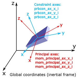
The three coordinate systems and their respective commands are shown in Figure 1.Figure 1. Coordinate Systems used for PASSIVE_RIGID_BODY and the Respective
Definition Commands. In general, it is not necessary for the three coordinate systems to
align.
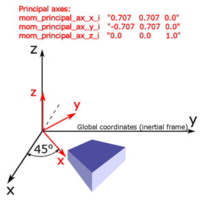
An example of a hexagonal body that is rotated by 45 degrees around the z axis in
Figure 2. Since it is easier in this case to specify the moment of
inertia with only diagonal terms, you will define a principal axes coordinate
system.Figure 2. Hexagonal Body Rotated by 45 Degrees around the Z-Axis. Appropriate commands are used to define the principal axes coordinate
system.
The exact same principle can be applied to the constraint coordinate system if you,
for example, want to constrain the motion of the body in the direction that is under
45 degrees with respect to the global x or y axes.
By default the origin of the constraint coordinate system is located at the center of
mass of the body. That is to say that if the body is to rotate, it will rotate
around its center of mass. However, there are a number of situations where this
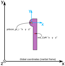
behavior is not suitable. One example is a simulation of a hinge. In a situation
like that, where you want the rigid body to rotate around a specific point, you need
to shift the coordinate center of the constraint coordinate systems. For this
purpose you can use the prbcon_pt_i command. Along with the new
coordinate center you need to set the rotational constraints for the new “hinge
point”. This is done using prbcon_ax_hinge_c command, where it is
a vector that says which rotational motions are locked (x, y or z axis in constraint
coordinate system). By setting all three values to 0 you will essentially define a
ball-joint. The simplified 2D setup of a hinge is shown in Figure 3.Figure 3. 2D Hinge. This example shows how to define a new coordinate center for the
constraint coordinate system using prbcon_pt_i command.
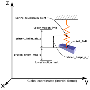
Linear or torsional springs can also be defined. To illustrate the basic concept of
such a setup, refer to Figure 4. The example shows the setup of a body which is hanging on a spring. The initial
location of the body does not correspond to the equilibrium point of the spring,
that is to say that you have a pre-deformation of the spring
(prbcon_linspr_p_c) when starting the simulation. Along with
this you of need to set the stiffness coefficient of the spring
(prbcon_angspr_k_c). Between these two parameters you can
define a force that is initially acting on the spring. Same principles apply for
torsional springs, except that the deformation is expressed in [rad], and the
stiffness of the spring in [Nm/rad].
There is also an option to set upper and lower coordinate (angle) bounds for the
body. In order to do so you must use
prbcon_linlim_pls_candprbcon_linlim_mns_c (or
prbcon_anglim_pls_candprbcon_anglim_mns_c for angular limits) to
define positive and negative displacement, respectively. These commands are always
defined with respect to the init_CoM.Figure 4. Linear Spring Setup with Annotated Commands
The linear commands for the above options all have their rotational counterparts
which can be found in the Motions section.
Note:
Rigid-rigid body or wall-rigid body interactions are not supported. It is
possible to simulate more than one rigid body in the domain, but their
interactions are not modeled.
Also, a rigid body cannot cross a PERIODIC boundary.
With passive rigid body motion it is also possible to prescribe constant force or
torque acting on a body by using prbcon_cnstfrc_c or
prbcon_cnsttrq_c.
Alternatively, you can prescribe either constant or varying linear or angular
velocities to each of the bodies by using prbcon_linvel_* and
prbcon_angvel_* sets of commands.