Create an Activate model that supplies a three-phase bridge current into a Flux 2D model
of a Surface Mounted Permanent Magnet (SPM) motor, and co-simulate the models.
Attention:Available only with Activate commercial edition.
The co-simulation process includes four basic steps:
Create a Flux model. For this tutorial, a Flux model of an SPM motor is provided for
you.
Generate the Flux coupling component required for Activate to read in the Flux model
data.
Create an Activate model and include the Flux block for reading in the Flux coupling
component.
Co-simulate the models in Activate.
Files for This Tutorial
SPM_Activate_Regulation.F2STA (the coupling file exported from Flux),
SPM_Activate_RegulationF2STA.FLU (the Flux model file), SPM_Regulation_No_load.scm (the Activate model
file)
A finished version of the models you build in the tutorials along with any files
required to complete the tutorials are available at this location:
<installation_directory>/tutorial_models/Flux_SPM.
Important: The co-simulation process requires that the FLUX
.FLU and .F2STA files be located in
the same working directory. When naming the working directory, avoid spaces and
special characters as Flux cannot recognize them.
Overview of the Flux SPM Motor
The Flux model is a brushless, AC, Surface Mounted Permanent Magnet motor applicable for
electric vehicles.
The SPM motor is comprised of three main components:
Fixed part (stator) including yoke, slots, and windings
Air gap
Moveable rotor with embedded magnets
The SPM motor is driven with a three-phase bridge current (the freewheeling diodes are
neglected). The constant speed operation of the motor at 1000 rpm with inverter driver is
simulated to yield motor torque, speed, position and phase current. The inverter switching scheme
is rotor-position dependant.
The inputs for the SPM motor are defined as multi-physical parameters and include:
I1: Physical quantities: μr, Bs, Br
I2: Electrical quantities: resistance, voltage, current
The outputs for the SPM motor are scalar I/O settings that retrieve values through the sensors,
formulas (forces and couples) and parameters (position, speed, acceleration).
The electrical circuit of the SPM motor is configured with a voltage source, coil conductor,
resistor, inductance, solid conductor and switch.
Note: Included in the switches are the input
parameters R1, R2, R3, R4, R5 and R6. The strategy is that each phase has to be "ON" for one
third of the period. For this model, the mechanical period is 180 degrees because the model is a
two-pair pole electrical machine.
Figure 1. Electrical Circuit of the SPM Motor
Generating the Coupling Component in Flux
Load the Flux model and generate the coupling component with the required inputs,
outputs and parameters.
Launch Flux, and from your working directory, open the project,
SPM_Activate_Regulation.F2STA.
The model loads and looks something like this:Figure 2. Cross-Section View of SPM Motor
From the Flux 2D toolbar, select Solving > Generate component for Activate coupling.
In the dialog, enter the following information for the component:
Enter the name for the component:
SPM_Activate_Regulation.
Enter the path to your working directory:
<name_without_spaces>.
Select the input (geometric I/O parameters) for the component:
R1, R2, R3, R4, R5, R6.
Select the output: PHASE_CURRENT_1, PHASE_CURRENT_2,
PHASE_CURRENT_3, POSITION, SPEED and
TORQUE.
The dialog should look something like this:
Click OK.
The coupling component is saved to your working directory as SPM_Activate_Regulation.F2STA.
Creating the Activate Model
Create a model to feed a three-phase bridge circuit.
From Activate, create a new model and save it to your working directory as
SPM_Regulation_No_load.scm
Alternatively, load the model:
<installation_directory>/tutorial_models/Flux_SPM/SPM_Regulation_No_load.scm and skip this section
of the tutorial.
From the Palette Browser, select Activate > CoSimulation, and drag and drop one Flux block into
your diagram.
Double-click the Flux block, and in the block dialog,
for Flux to Activate input filename, enter the path to
the coupling component you generated from Flux:
<working_directory>/SPM_Activate_Regulation.F2STA.
Click OK.
The Flux block populates with the model data from the Flux coupling
component.
On the Flux block dialog, do the following:
For Numerical memory (MB), enter 2154.
For Character memory, enter 200.
For Minimal input variation %, enter 0.
Select the options: Flux console display and
Break algebraic loop.
Click OK.
The Flux block dialog should look something like this:
In the diagram, to the left of the Flux block, create a super block for
Position regulation:
Table 1. Blocks Required for Position Super Block
Add these blocks to the super block
Enter parameter values or keep default values as
indicated
1 Constant block
Default
1 Modulo block
Function = Remainder
1 Input block
Note: The Input block (Rotor position) feeds
into the Modulo block.
Outport size = [-1;-2]
1 LastInput block
Default
2 Sum blocks
Default
8 LookupTable blocks
For all 8 LookupTable blocks:
Y =
[1,1]
Interpolation
method = ZeroOrder
(ceiling)
Output datatype =
"double"
For the X vector, enter:
block 1, X =
[15,75]
block 2, X =
[45,105]
block 3, X =
[75,135]
block 4, X =
[105,165]
block 5, X
= [0,15]
block 6, X =
[135,180]
block 7, X
= [0,45]
block 8, X =
[165,180]
2 Sum blocks
Default
6 Output blocks
Note: The Output blocks correspond to the
6 input ports "R1" through "R6" of the Flux block in the
main diagram.
Default
Scope
Default
Assemble the blocks in the super block like this: Figure 3. Position Super Block
In the diagram, add three Scope blocks to the right of the Flux block. The
Scope blocks plot the following results: current (A) in each phase, position and
speed, and torque.
Define
Scope 1
Scope 2
Scope 3
Block name
2_1_2
2_1_2_1
2_1_2_1_1
Number of inputs
3
2
1
Assemble and connect the Flux co-simulation block, super block and scope blocks
as you see in the following figure, and save the model.
Figure 4. Flux Block Assembled with Inputs and Outputs
The Activate model is now complete and configured to supply the Flux model of
the SPM motor with a three-phase bridge circuit. The Activate model is also
configured to calculate the phase current, position, speed and torque.
Co-Simulating the Activate and Flux Models
During co-simulation, the Activate model supplies a three-phase bridge current into
the Flux model of the SPM motor. The simulation results show the performance of the SPM
motor including position, speed and torque.
On the ribbon, select Setup.
On the dialog that appears, select the Simulation Time
tab.
For Final Time, enter .01499, which is the signal
period. Keep the defaults for the remaining fields.
Select the Solvers tab, enter the following values, and
click OK:
On the ribbon, select Run.
The simulation results show the currents fed into the motor and the
motor performance.
Table 2. No Load Test with Constant Speed (N=1000 rpm)
Property
Value
Unit
Moment of inertia
0
Kg.m2
Constant friction coefficient
0
N.m
Viscous friction coefficient
0
N.m s/deg
Friction coefficient proportional to the square
speed
0
Speed
1000
Tr/min
Position at time 0
0
Deg
Figure 5. Current (A) in Each PhaseFigure 6. Position (deg/s) and Speed (rpm)Figure 7. Torque (N.m)
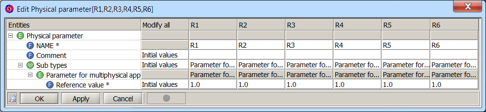
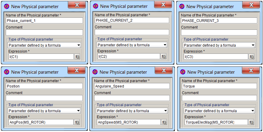
 Figure 1. Electrical Circuit of the SPM Motor
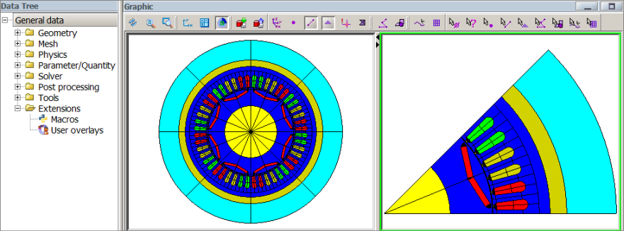 Figure 2. Cross-Section View of SPM Motor
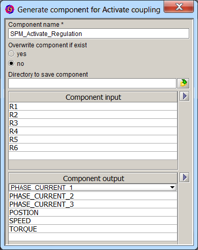
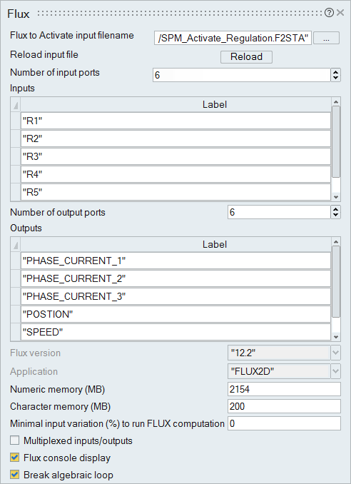
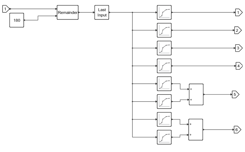
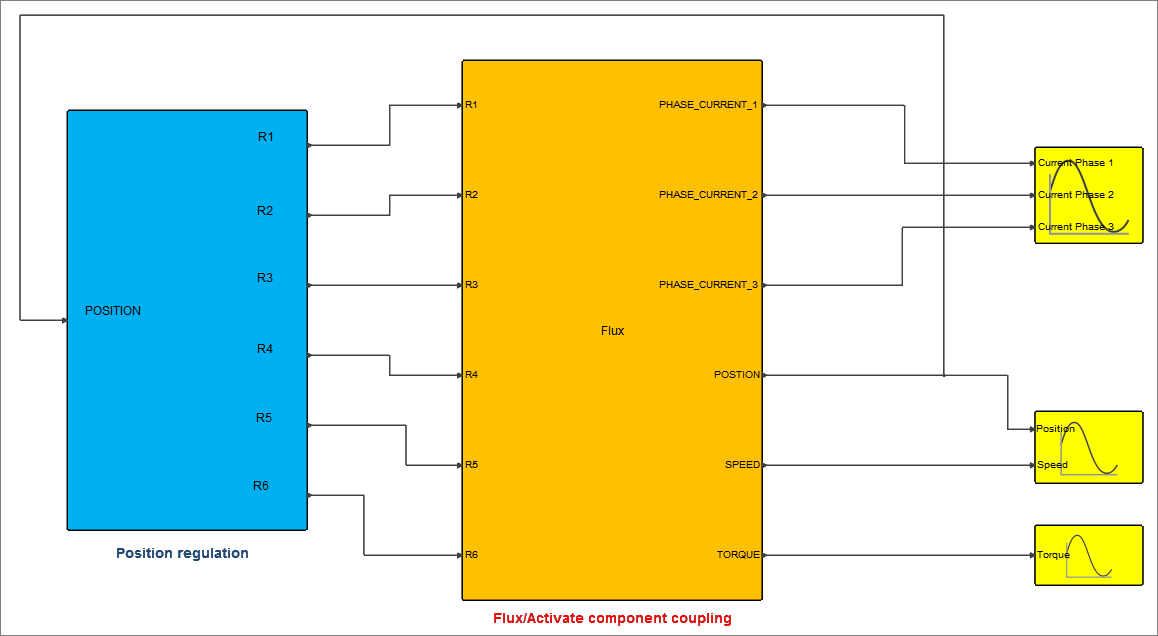 Figure 4. Flux Block Assembled with Inputs and Outputs
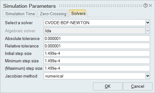

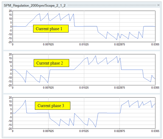
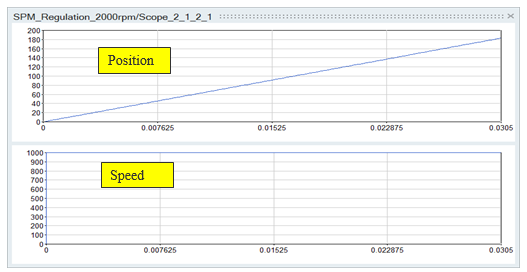 Figure 6. Position (deg/s) and Speed (rpm)
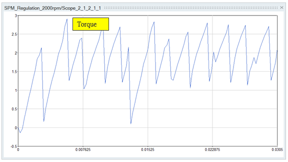 Figure 7. Torque (N.m)