Example 3
In this example, the Monostatic RCS of two cubes is calculated, where one cube is dynamic.
Step 1
Create a new project following steps 1 to 5 in Example1 above.
Step 2
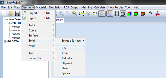
Click on Geometry → Solid → Box.
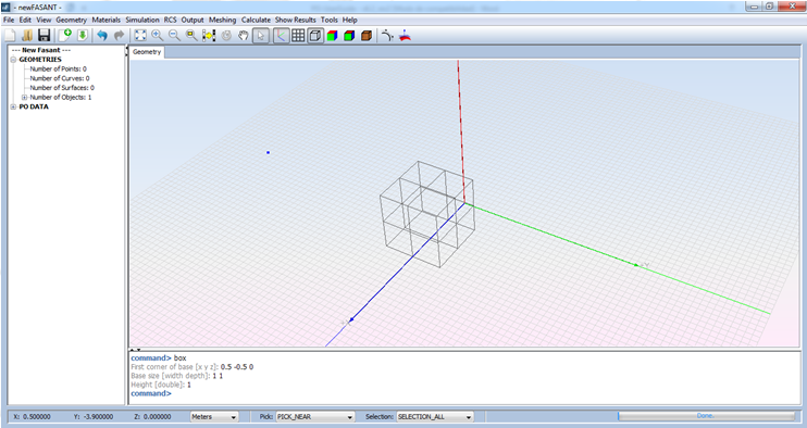
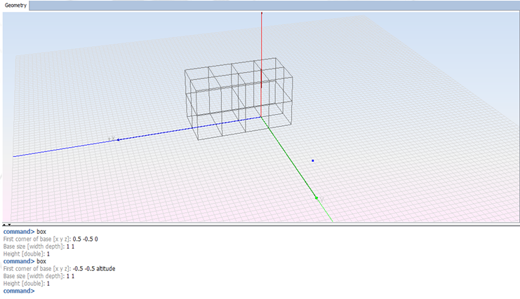
Create the first box by entering the following parameters from the command line as shown in the next Figure.
· First corner of base [x y z] 0.5 -0.5 0
· Base size [width depth] 1 1
· Height 1
Step 3
Now, let’s add the dynamic cube to the model. We want this cube to move in the direction of the positive Z-axis at 0.5 meters each step in the simulation. We will use three steps for this simulation.
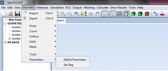
First, we must define a parameter for the geometry that represents the Z coordinate of the base of the cube at each step of the simulation. To do this, select Geometry → Parameters → Define Parameters and the following window appears:
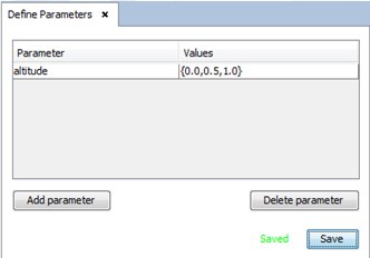
Press the Add parameter button, after which a row appears in the table. In the Parameter column, change the name of the created parameter to “height”, for example. Then change the values to “{0.0, 0.5, 1.0}” and left-click the Save button to save the changes.
Now, create a new box as the other. It is possible to change the parameters as desired, but the z coordinate of the first corner of the base must be now the parameter “altitude”.
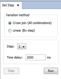
Optional: To see a visualization of each step for the second cube, select the Geometry → Parameters → Set Step. Enable “Linear (By step)”, set the desired time delay between steps, and left-click Run to see the animation on the Geometry View.
It is possible to see the two remaining steps for the simulation in the next Figures.
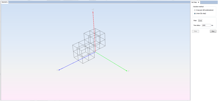
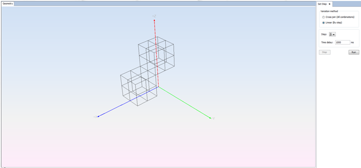
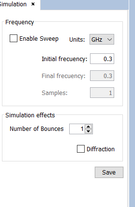
Step 4: Click on Simulation → Parameters. Enter the simulation parameters as shown in the next Figure.
Step 5
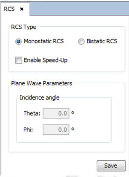
Select RCS → Parameters and enter the parameters shown in the next Figure.
Step 6
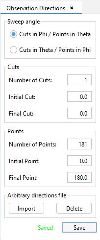
Select Output → Observation Directions and enter the parameters shown in the next Figure.
Step 7
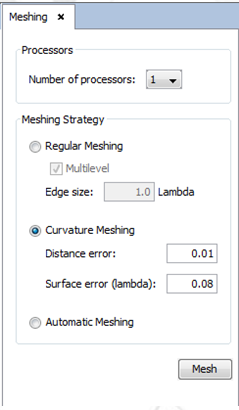
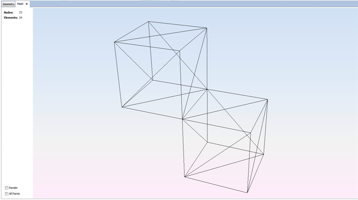
Select Meshing → Create Mesh. Select the appropriate number of processors available to run the meshing process as shown in the next Figure and left-click Mesh.
Step 8
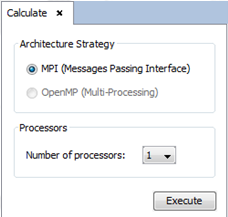
Select Calculate → Execute and enter the number of available processors for this simulation.
Step 9
Click on Show Results → Far Field → View Cuts, to show the RCS graph.
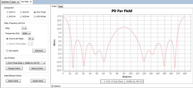
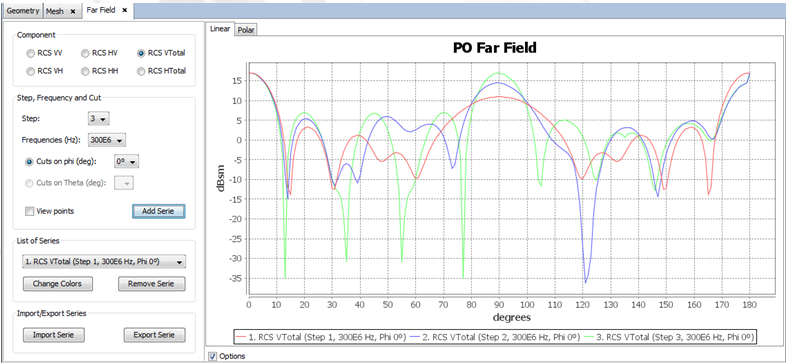
The plot corresponds to the RCS of the first step (when the two boxes share the same Z coordinate). To plot the graphics for the remaining two steps, select “2” in the Step combo-box and left-click the Add Series button. Repeat this procedure to add Step 3 to the RCS graphic.
Step 10
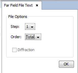
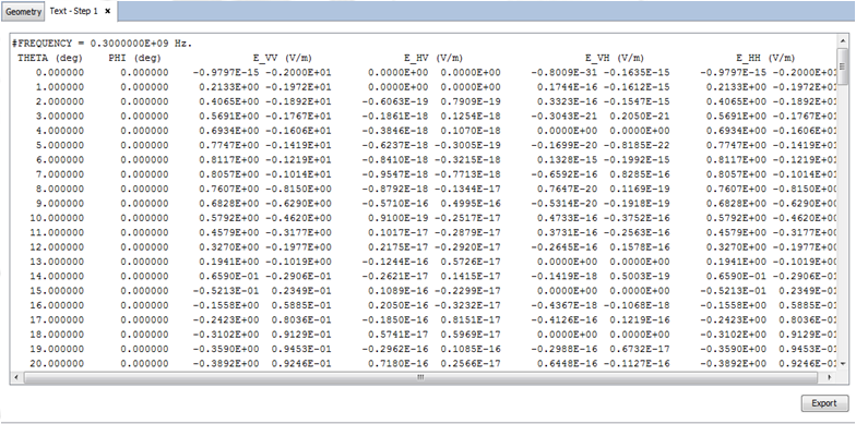
Click on Show Results → Far Field → View Text Files, to show the RCS data file. Select the step to obtain as a data file. Press OK to continue.
