In this example, the Monostatic RCS of a plane is calculated. The normal vectors of
the geometry are duplicated for this simulation.
Step 1
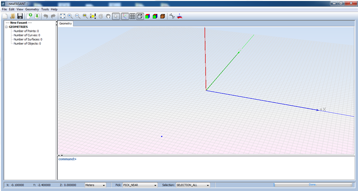
Start newFASANT.Figure 1. Start newFASANT window
Step 2
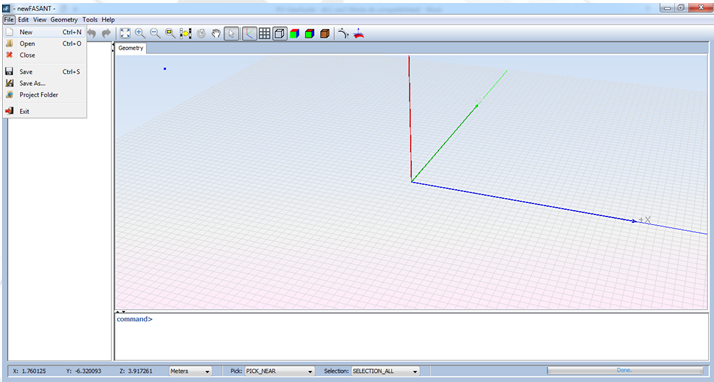
Select File and click on New.Figure 2. New File
Step 3
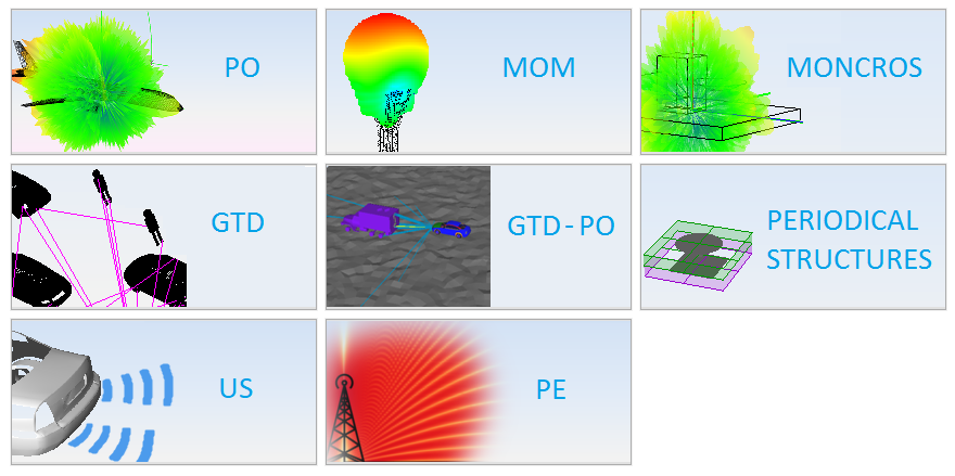
Select PO.Figure 3. Method Type selection
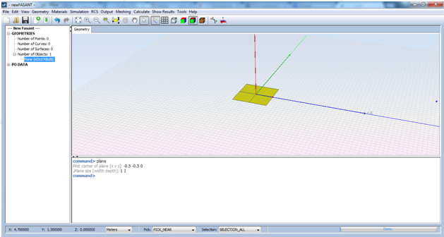
Step 4
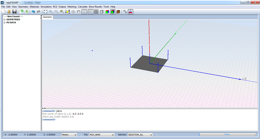
Click on Geometry → Surface → Plane, which introduces the first and the second point
dialog as shown in the next Figure.
In this example the user enters the following parameters into the command line:
First corner of plane: -0.5 -0.5 0
Plane size [width depth]: 1 1
Figure 4. Create plane command
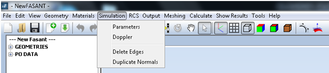
Step 5
Click on Simulation → Parameters.Figure 5. Simulation Parameters Menu
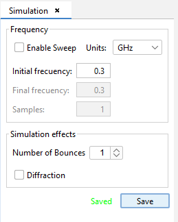
Step 6
Select 1 bounce (simple reflection) and a frequency of 0.3 GHz as shown and
left-click the Save button.Figure 6. Simulation Parameters panel
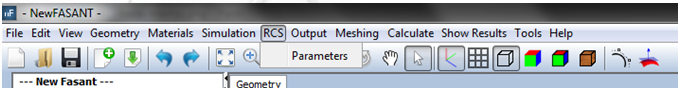
Step 7
Select RCS → Parameters.
This command appears in the top left side of the newFASANT window as shown in the next Figure.Figure 7. RCS Menu
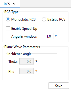
Step 8
Select Monostatic RCS only, and left-click on the Save button.Figure 8. RCS Parameters panel
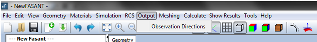
Step 9
Select Output and left-click on Observation Directions.Figure 9. Observation Directions Menu
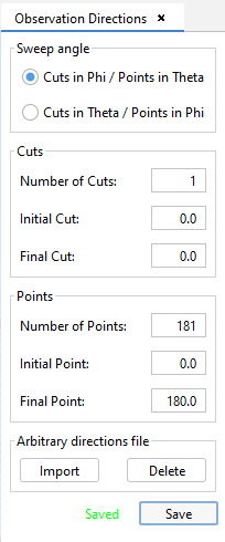
Step 10
Introduce the far-field observations (cuts, points and sweep angles), as shown in the
next Figure and left-click on the Save button.Figure 10. Observation Directions panel
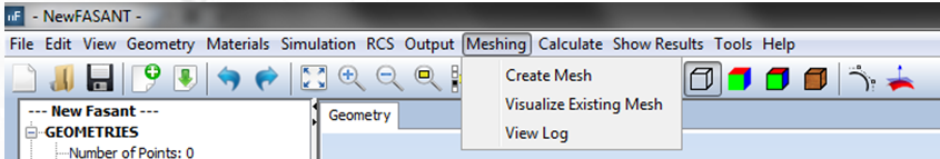
Step 11
Before running the case, select Meshing → Create Mesh.Figure 11. Meshing Parameters Menu
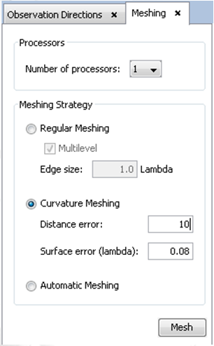
Step 12
Select 1 processor and define the curvature mesh option with a distance error of 10
and surface error of 0.08 and left-click on Mesh.Figure 12. Meshing Parameters panel
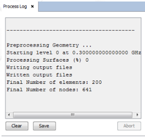
Left-clicking on Mesh enables the meshing engine as shown in the next Figure:Figure 13. Mesh process
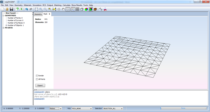
In order to visualize the mesh, then Meshing → Visualize Existing Meshing and select
the .msh file.Figure 14. Mesh visualization
Step 13
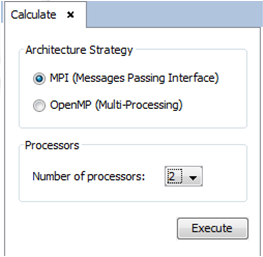
Select Calculate → Execute and then indicate the a number of processors available to
simulate this case.Figure 15. Execute panel
Figure 16. Execute information
Step 14
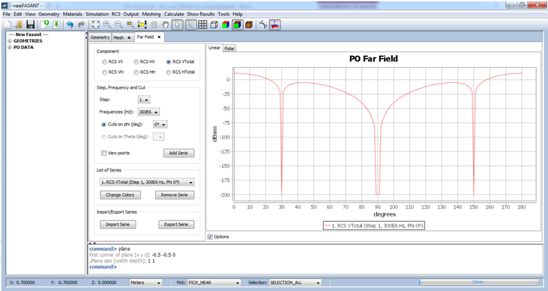
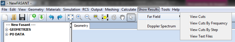
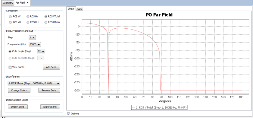
When the simulation finishes, we can visualize the simulation results. Click on Show
Results → Far Field → View Cuts, which allows the user to show the RCS graphic (in
the next figure).Figure 17. Far Field View Cuts Menu
Figure 18. RCS Graphic
Step 15
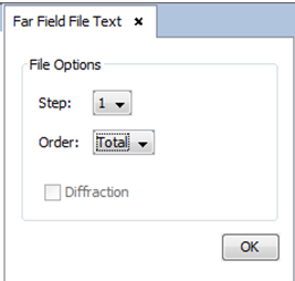
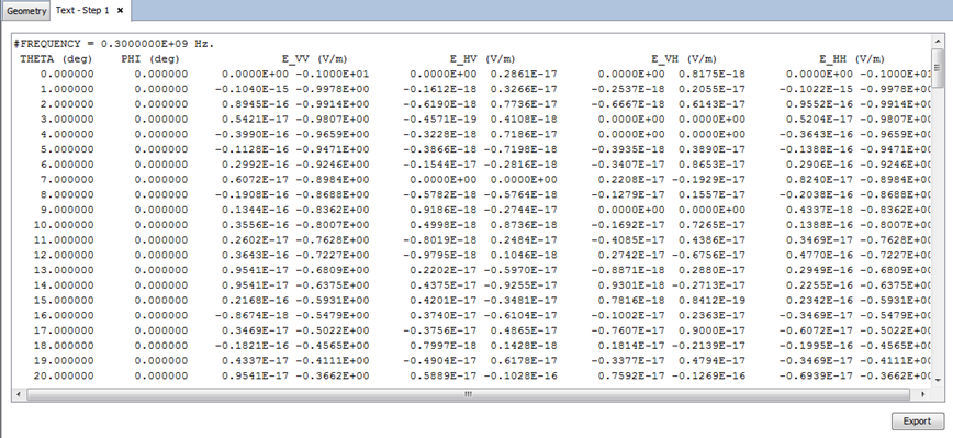
Click on Show Results → Far Field → View Text Files. Then select the Steps and the
order and press OK to show the RCS data file.Figure 19. Far Field View Text File panel
Figure 20. Result Text File visualization
This example has been executed using a plane whose normal vector is along the Z-axis.
The user can duplicate this vector and simulate the problem again using duplicate
normal vectors. After the simulation, the user can visualize the results to
see the differences between one normal vector and two duplicated normal vectors. To
view the normal vectors of this geometry, click the icon, as shown in the next
Figure.Figure 21. Appearance Normals visualization
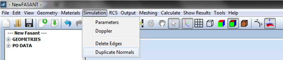
Step 16
To duplicate the normal vectors click on Simulation → Duplicate Normals.Figure 22. Duplicate Normals Menu
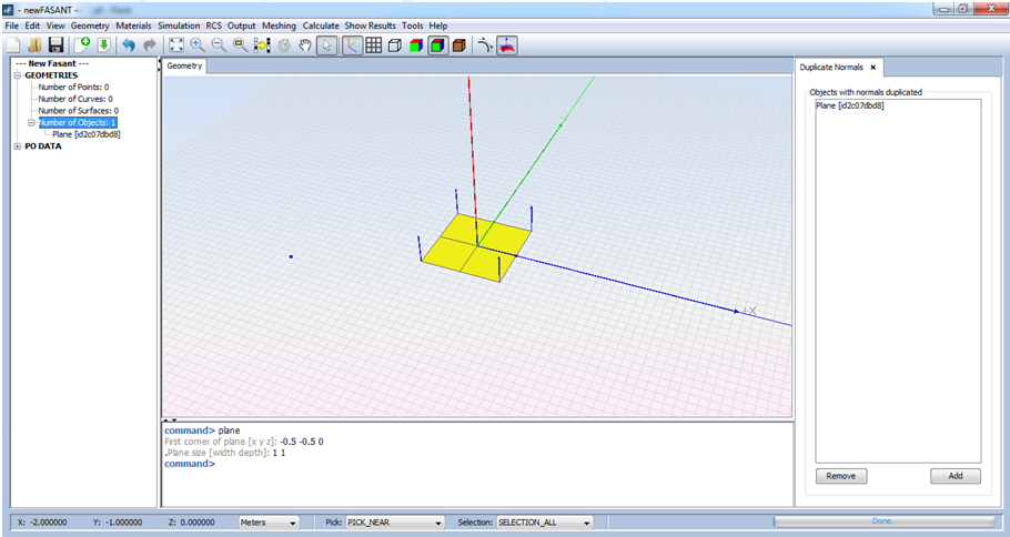
Then select the object to duplicate the normal vector and left-click the Add button
in the right panel that has appeared.Figure 23. Duplicated Normals visualization
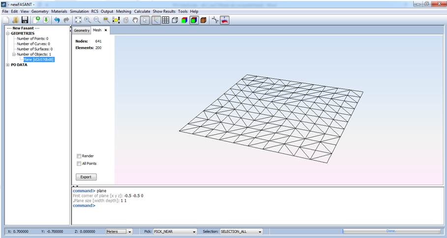
Step 17
Re-mesh the geometry and start the simulation again, like in step 12 and 13. The
process is simply the same.Figure 24. Mesh window
Step 18
Click on Show Results → Far Field → View Cuts, to show the RCS graphic like in step
14. In this case, we can notice that the result is different.Figure 25. RCS Graphic
 icon, as shown in the next
Figure.
icon, as shown in the next
Figure.