Example 2: Design and Analyze a Conical Corrugated Horn at 10 GHz and 22 dB Gain
This case explains how to calculate far-field, radiation pattern, current density, charge density and near field of a corrugated horn with 22 dB gain at 10 GHz.
Step 1: Create a new MOM Project.
Open newFASANT and select 'File --> New' option.
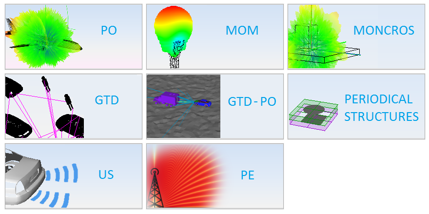
Select MOM option on the previous figure and start to configure the project.
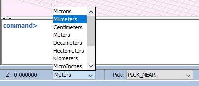
Step 2: Change the scale to millimeters.
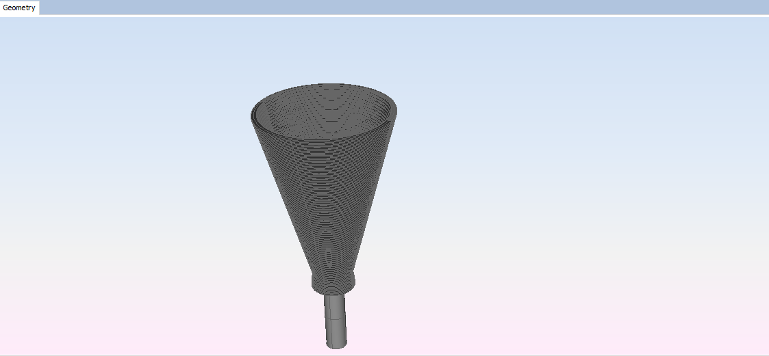
Step 3: Create the geometry of the corrugated horn.
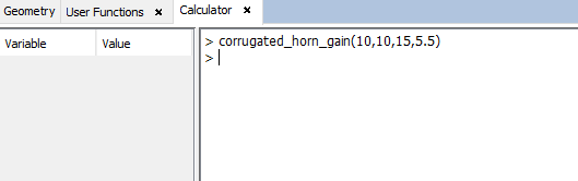
Execute the function “corrugated_horn_gain(fmin,fmax,alfa,D)". To execute the function, click on Tools - Calculator and write the call to the function.
- fmin is the lowest operating frequency (GHz)
- fmax is the highest operating frequency (GHz)
- alfa is the flare angle (obtained from the following graph)
- D is the aperture diameter (obtained from the following graph)
In this case, we will simulate at 10 GHz, so the maximum and minimum frequency are 10 GHz.
To choose the flare angle and the aperture diameter, observe the next graph.
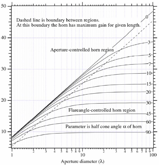
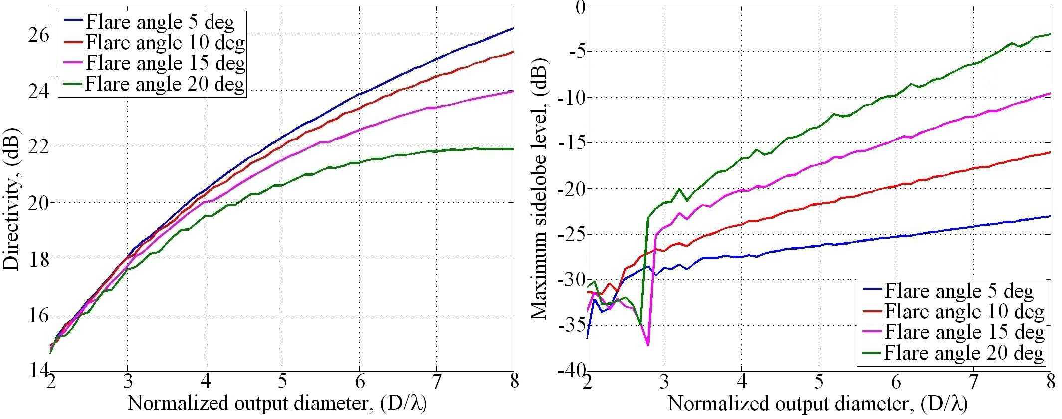
- Alpha = 15
- D = 5.5
The script file, called “ script_corrugated_horn_gain.nfs”, will be automatically generated in the mydatafiles folder in the newFASANT directory.
The next step is to execute the generated script file. For that, click on Tools – Script - Load and open the script script_corrugated_horn_gain.nfs.
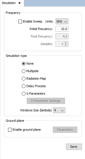
Step 4: Set Simulation Parameters
Select 'Simulation --> Parameters' option on the menu bar and the following panel appears. Set the parameters as the next figure shows and save it.
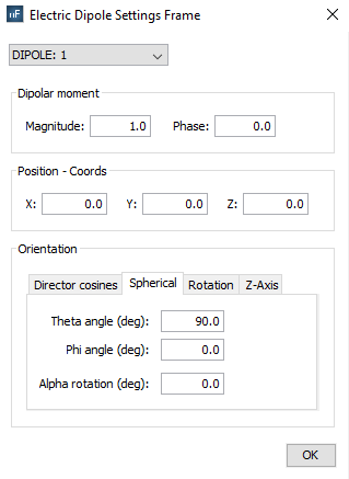
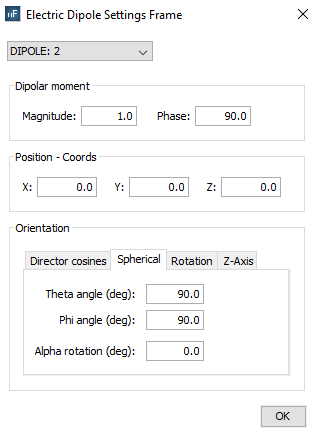
Step 5: Set the source parameters.
Select 'Source --> Dipole --> Dipole Antenna' option and set the parameters as show the next figure. Then save the parameters and the dipole appears.
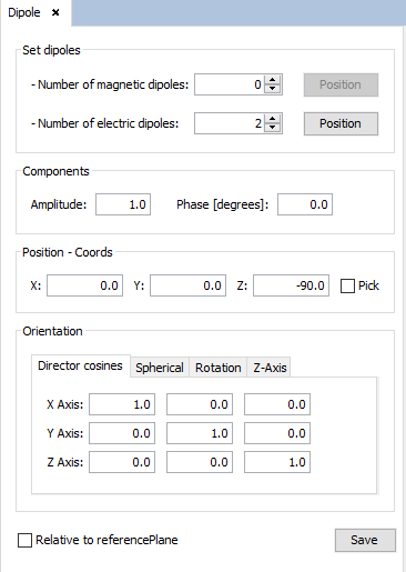
Select 2 electric dipoles and click on “Position”.
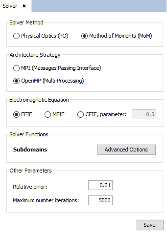
Step 6: Set the solver parameters. Click on Solver --> Parameters option on the menu bar. Verify that all the parameters are defined by default, as shown in next figure. Click on Save button before going to next step.
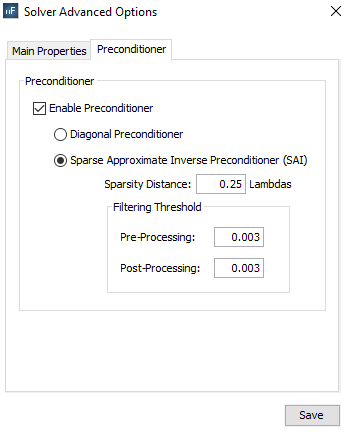
Select ‘Advanced Options’ and activate Preconditioner as shown.
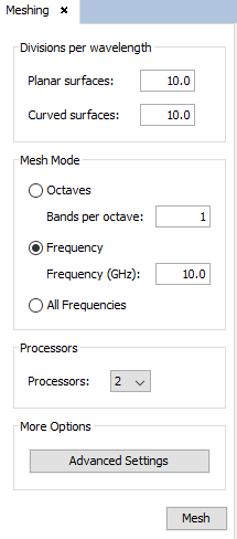
Step 7: Meshing the geometry model.
Select 'Meshing --> Parameters' to open the meshing configuration panel and then set the parameters as show the next figure. In order to obtain the shortest possible time for meshing, it is recommended to run the process of meshing with the number of physical processors available to the machine.
Step 8: Execute the simulation.
Select 'Calculate --> Execute' option to open simulation parameters. Then select the number of processors as the next figure show. In order to obtain the shortest possible time for calculating the results, it is recommended to run the process with the number of physical processors available to the machine.
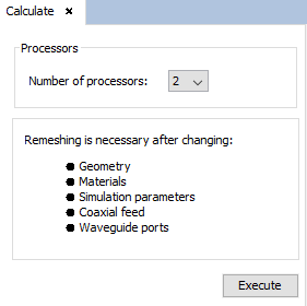
Then click on 'Execute' button to starting the simulation.
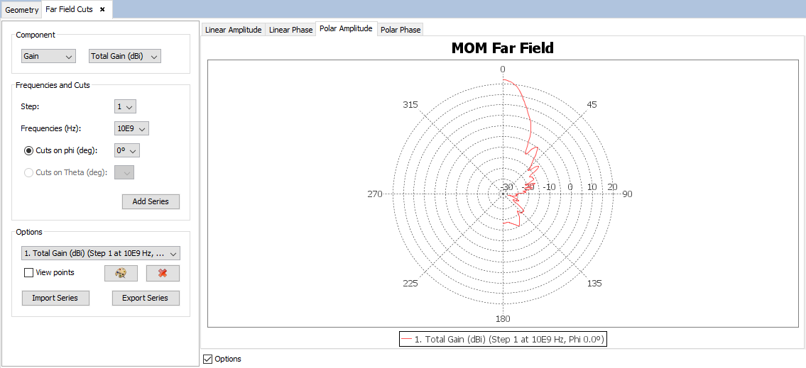
Step 9: Show Results.
To get more information about the graphics panel advanced options (clicking on right button of the mouse over the panel) see Annex 1: Graphics Advanced Options.
Select 'Show Results --> Far Field --> View Cuts' option to show the cuts of the observation directions options.
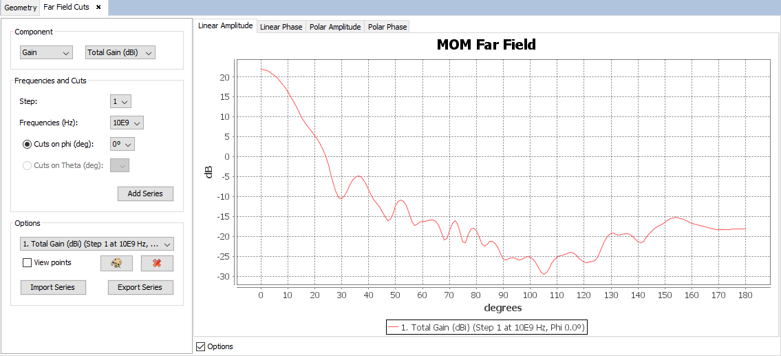

Selecting other values for the component, step, frequency or cut parameters and clicking on 'Add Series' button a new cut will be added to the selected parameters.
On 'Show Results --> Far Field' menu, other results are present such as 'View Cuts by Step' and 'View Cuts by Frequency' and this option display the values for one selected point for each step or frequency.
Select 'Show Results --> Radiation Pattern --> View Cuts' option to show the cuts of the radiation pattern options.
Selecting other values for the component, step, frequency or cut parameters and clicking on 'Add Series' button a new cut will be added to the selected parameters.
On 'Show Results --> Radiation Pattern' menu, other results are present such as 'View Cuts by Step' and 'View Cuts by Frequency' and this option display the values for one selected point for each step or frequency.
Select 'Show Results --> Radiation Pattern --> View 3D Pattern' option to show the cuts of the radiation pattern options.
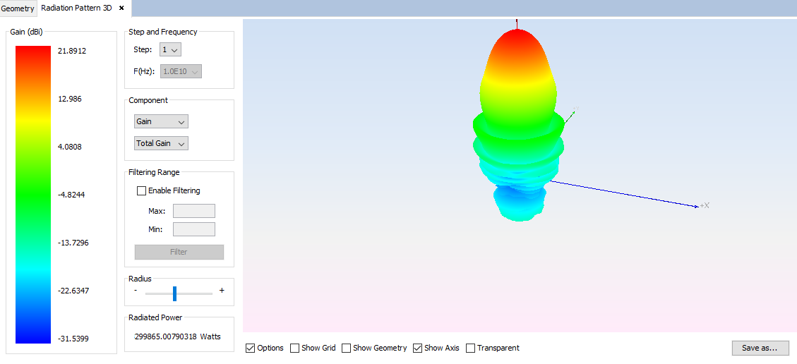
Changing values for step, frequency, component or filtering parameters the visualization for the new parameters will be shown.
Select 'Show Results --> View Currents' option to show the current density.
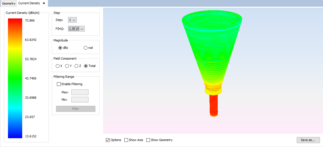
Changing values for step, frequency, magnitude, component or filtering parameters the visualization for the new parameters will be shown.
Select 'Show Results --> View Charges' option to show the charge density.
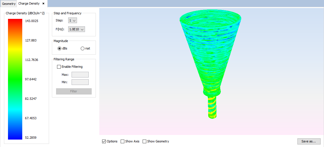
Changing values for step, frequency, magnitude or filtering parameters the visualization for the new parameters will be shown.
On 'Show Results --> Far Field' menu, other results are present such as 'View Cuts by Step' and 'View Cuts by Frequency' and this option display the values for one selected point for each step or frequency.