Automatic Report Generation Examples
Use hwGenImages to create a .pptx or .pdf report with user defined visualization.
Create a Simple Input File
DATASET{
     type                  	= ufx
     ufx_file              	= "./uFX_fullData/uFX_output.layout"
     summary_file          	= "./uFX_summary.txt"
}
COVER_PAGE{
     title_text             	= "Altair Roadster"
}
DISPLAY{}
Each command here starts with the name, COMMAND, followed by curly
braces {} with options specified inside the braces. The simulation
data to summarize is specified with the DATASET{} command. The
cover page settings are under COVER_PAGE{}. The title is set to
“Altair Roadster”. The DISPLAY{} sets document
properties with default values.
>> hwGenImages -pb report -no_run
 Figure 1. |
 Figure 2. |
Add Images
IMAGE{} command to tell the utility to create and display an
image. In the command options, specify which parts are to be shown and the views
from which the image is to be rendered. In this example, we define two views:
front-top-left and left.IMAGE("Fan_view"){
parts = {"Fan"}
views = {"front_top_left","left"}
image_type = static
}PART{} command. This particular command instance is named
Car and is referenced above with this name. A PART{} command
includes all boundaries and default visualization settings. These are optional and
can be customized as seen
below:PART("Car"){
show_boundary_names = {"_all"}
display_type = solid
solid_display_type = smooth
color_type = constant
constant_color = "white"
}COVER_PAGE{
title_text = "Fan: Without Duct"
cover_image = "Fan_view"
cover_image_view_number = 1
}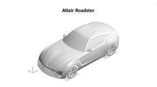
Figure 3.
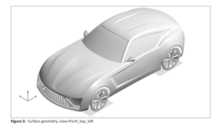 Figure 4. |
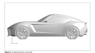 Figure 5. |
Results Visualization Tools
Using the advanced options enables you to unlock more colorful possibilities. Visualization mainstays such as Contours, Cut-planes, Iso-surfaces, and Streamlines have dedicated commands. Two-dimensional plots such as Line-plots and Bar-charts can also be created. All these commands can be further customized using the VARIABLE{} command that makes these commands more powerful and portable across multiple simulations. Last but not the least, two simulation results can be used to create a report that renders images side by side for a quick spot the difference comparison.
Surface Contours
color_type from constant to contour. This changes the
coloring of the car model from a constant color to a surface contour. We also
specify the contour function which controls the coloring of the contour, in this
example time_avg_Cp. This is followed by more settings that control
the legend on the right hand corner in the
plot.IMAGE("Surface Cp"){
parts = {"Surface Cp"}
views = {"front_top_left"}
image_type = static
}
PART("Surface Cp"){
display_type = solid
solid_display_type = smooth
color_type = contour
contour_function = time_avg_Cp
constant_color = "white"
legend_display = on
num_labels = 2
legend_use_local = off
legend_min = -0.5
legend_max = 0.5
num_decimal_places = 3
}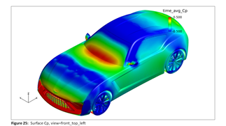
Figure 6.
Cut Planes
y = 0 is
defined. The instantaneous velocity magnitude, inst_velocity_mag,
is used to color the plane and the size of the plane is controlled by the inputs:
x_min, x_max, and z_max.car_length and
car_height are needed for the command to
work.IMAGE("Cut plane y inst. vel"){
cut_planes = {"y cut vel_inst"}
parts = {"Full vehicle - white"}
views = {"left"}
clip_parts = off
}
CUT_PLANE("y cut vel_inst"){
normal_direction = y
cut_location = 0.0
display_type = solid
solid_display_type = smooth
color_type = contour
contour_function = "inst_velocity_mag"
contour_line_display = off
contour_line_display_type = "constant"
mesh_line_display = off
constant_color = black
line_thickness = medium
legend_display = on
legend_use_local = off
legend_min = 0.0
legend_max = 45.0
num_labels = 5
num_decimal_places = 1
x_min = -0.78 - car_length/4.0
x_max = 3.29 + car_length
z_max = 1.3 + 0.5*car_height
}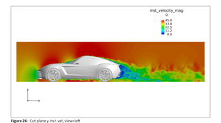
Figure 7.
Variables
variable_name, and an expression associated
with it. The expression can be a constant, another variable, or a mathematical
expression containing more variables. The following variables,
car_length and car_height need to be defined
to get the CUT_Plane{} in the previous section to work
correctly.VARIABLE{
variable_name = car_length
expression = 4.07
}
VARIABLE{
variable_name = car_height
expression = 1.317
}Iso-Surfaces
time_avg_velocity_x, is used to create the iso-surface which is
then colored with another variable, time_avg_Cp. If the iso-surface
needs to be painted with a constant color, set color_type to
constant and set constant_color to a supported
color (for example, white or
magenta).IMAGE("X Velocity = 0"){
parts = {"Full vehicle - white"}
iso_surfaces = {"X Velocity = 0"}
views = {"rear_top_left"}
image_type = static
}
ISO_SURFACE("X Velocity = 0"){
iso_function = time_avg_velocity_x
iso_value = 0
display_type = solid
solid_display_type = smooth
color_type = contour
contour_function = time_avg_Cp
legend_display = on
num_labels = 2
legend_use_local = off
legend_min = -0.5
legend_max = 0.5
transparency = 0
legend_display = on
num_labels = 2
legend_subtitle = ISO of X Velocity = 0
num_decimal_places = 1
}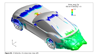
Figure 10.
Line Plots
data_file input. The data in the
ASCII file is organized
into rows and columns. Specify the column numbers in the x_column
and y_column fields to get a line
plot.LINE_PLOT("Instantaneous drag"){
data_source = "file"
data_file = "./uFX_coefficientsData/uFX_coefficients_Inst.txt"
num_header_rows = 11
x_column = 1
y_columns = {2}
x_label = "Time (s)"
y_label = "Coefficients"
title = "Instantaneous Drag"
legend_labels = "C_d"
show_legend = on
show_grid = on
}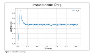
Figure 11.
Compare Simulations
Multiple simulations can be compared in a single powerpoint document. This is
especially useful when minor modifications to a model need to be tested and
visualized. In this example, a car with and without mirrors is compared. To request
a comparison, a REPORT{} command with the input
report_type set to run_comparison. Specify the
location of the second set of simulation images with
comparison_image_dir. This is in addition to the primary
DATASET{} command. A side_by_side comparison
will generate a report where all plots and images are placed side by side for
comparison. A flip book style comparison where images are placed one after another
in two pages can be generated with the run_comparison_type set to
woven.
REPORT("with and without mirrors advanced"){
    report_type          = run_comparison
    format	             = powerpoint
    image_borders	     = off
    comparison_image_dir = "../02/IMAGES-1.DIR"
    case_1_title         = without mirrors
    case_2_title         = with mirrors  #  title for the data in comparison_image_dir = ...
    slide_aspect_ratio   = "16:9"
    run_comparison_type  = side_by_side
}
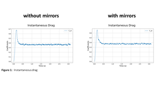 Figure 12. |
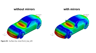 Figure 13. |