FMI (Functional Mock-up Interface)

Introduction

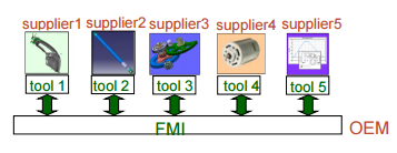
Automotive OEMs, who may have several hundreds of suppliers, have difficulties when they need to integrate many sub-systems from those suppliers.

Since they are specialized subsystems, such as hydraulics, mechanical, and electrical, the suppliers use different modeling and simulation programs for developing their sub-systems or components. In order to make sure that all of these subsystems work actually all together, the OEM should simulate them all together and in combination. For that, the system integrator should be able to work with all programs and programs should be able to work with others. This is not only a problem in the automotive industry but it is prominent in this industry.

A solution would be to share the source code of models and compile them in the host simulator, but very often these models have proprietary rights and can only be delivered in binary form or as libraries, which means they need special tools.

Co-simulation between simulators is a popular solution to make simulators work together in parallel. This solution works to some extent. In order to implement a co-simulation interface between simulators, a specialized interface should be developed. That means an interface per every two simulators. There are many tools and it is usually very hard to replace one by another or do all simulations in a single tool. There are some programs specialized in Co-Simulation that can interface several simulation tools with several versions, but it is not practically easy to interface all simulation tools.

Developing export and import facilities to exchange models between tools seems also to be a good solution, but that needs developing special export and import between tools. Also, imported models do not usually work as well as in the original simulator due to differences in the simulator characteristics and lack of a standard format. There are several well-known interface formats, such as Modelica language, s-function from MathWorks, user routines in ADAMS, etc. But most of them are proprietary and cannot be used as standard for communicating between tools.

Even though Modelica is a tool independent language, it cannot be used as a standardized interface for model exchange because it needs a compiler to convert the language into the executable code.

In 2008, a large number of software and automotive companies as well as several European research centers worked in a cooperation project named MODELISAR to create the FMI (Functional Mock-up Interface) standard. (More information, detailed interface specification, and images used here can be found at www.fmi-standard.org.) The development of the FMI specifications was initiated and coordinated by the Daimler AG company. The FMI standard defines a general interface to other simulators. A component (model) which implements this interface is called FMU (Functional Mock-up Unit). The goal of FMI is that the calling of an FMU in a simulation environment becomes standardized and remains reasonably simple. The FMI functions can be imported and called by any external simulation environment such as Twin Activate. The host environment can create one or more instances of the FMU and simulate them. This is very similar to the way a model composed of several blocks can be created and simulated in Twin Activate. An FMU may either need a simulation environment to import it and perform numerical integration (FMI for Model Exchange) or have its own solvers/simulator (FMI for Co-Simulation).

In 2010 the first version of FMI-1.0 for Model Exchange and for Co-Simulation was released^{1, 2}.

In 2014, FMI-2.0 standard including both Model Exchange and Co-Simulation, was released³. FMI-2.0 fixed few issues in FMI-1.0 and is not backward compatible with FMI-1.0.

In 2022, the FMI-3.0 standard was released. The new features that are used or implemented in Twin Activate are:

Introduction of Clocks to more exactly control timing of events and evaluation of model partitions across FMUs.
Introduction of more integer types (signed and unsigned 8-bit, 16-bit, 32-bit, and 64-bit).
Introduction of a binary type to support non-numeric data handling, such as complex sensor data interfaces.
Extension of variables to arrays for more efficient and natural handling of non-scalar variables.
Introduction of structural parameters that allow description and changing of array sizes.
To allow implementation of more robust and efficient co-simulation algorithms, a few new features such as Event-mode have been added to FMI for Co-Simulation.

FMI Interface Types

The FMI standard, which was introduced to cope with tool interface problems, provides two major solutions for interfacing tools:

Interface as Model Exchange (in this topic often abbreviated as ME): FMI standardizes the model export as binary or as source code. In this interface type the model can be a system of algebraic-differential equations (at most index-1 DAE) with discrete equations. With this approach a large range of transient dynamical systems can actually be modeled. In this approach, the numerical solver which is external to the model should be compatible with the model. This interface type will be discussed more in FMI for Model Exchange (ME).
Figure 1. FMI for model exchange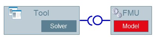
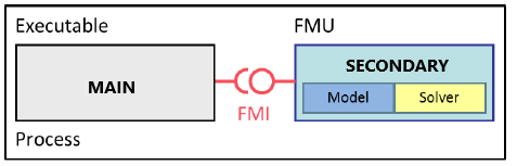
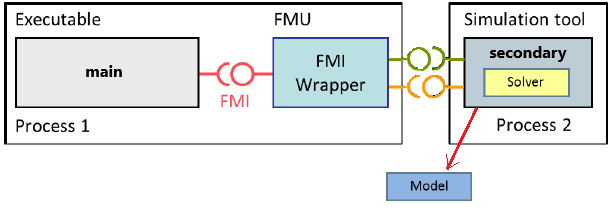
Interface as Co-Simulation (in this topic often abbreviated as CS): FMI standardizes the co-simulation between simulation tools. In this interface type, the FMU can contain the model, the numerical solver, and the simulator. It is also possible that FMU only provides the link between two tools without containing the solver or simulator. In this approach, the tool that imports the FMU, provides the input to the FMU and receives the output of the FMU. This approach is more general and any kind of simulator and any format such as physical models, 1D-3D and 0D for Controls can be interfaced. This interface type will be discussed more in FMI for Co-Simulation (CS).
Figure 2. FMI for co-simulation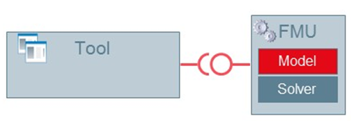

Advantages of Using FMI in Industry

FMI is a free and open standard published under a BSD license and currently supported by most important actors in the simulation software domain. Up to now, more than 70 tools support this standard according to the FMI-standard webpage. Both FMI interface types allow preserving the intellectual property of the supplier over the exported model. FMI-compliant tools often allow export of models freely licensed for distribution in the organization or to partners. As a result, exported FMUs most often do not require an extra license from the export tool to be accessed or executed (except for FMI for Co-Simulation with external solver where the remote simulator is still required). In industry, there are always only a handful of specialists on modeling who develop detailed high-fidelity models using modeling tools. They develop the model and deliver it to a large number of users who exploit the model for other applications such as:

Model parameter identification
Model sizing
Controller design
Model-specific analysis such as frequency analysis
Pre- and post-processing

None of these applications needs the modeling tool, which very often requires a costly license and good knowledge to use. In this situation, it is extremely useful to embed the model in an FMU and share it with other users. The FMU or model can be deployed from simulation specialists to designers, domain specialists, or control engineers in other departments. That is the advantage of FMI: less costly modeling tools and less expensive execution tools. As an example, consider the model of the engine developed by the mechanical engineering department. This FMU can be deployed to the electrical department for ECU design, to the thermal department for thermal requirements verifications, or to the control department for design-appropriate controllers. In each of these departments, several engineers can work on the same FMU with different FMI-compliant tools and each engineer can run several variants of FMUs at the same time.

An FMU can be used by different groups in different domains, i.e., multi-domain collaboration. Engineers in different domains such as mechanical, electrical, system, control, fluid, and thermal can work together with FMUs. They can share FMU models while staying with their tool of choice. Now, with the advent of a new standard, every tool supporting FMI can virtually be connected without developing a new interface.

It is important to highlight that the FMI is basically developed for system-level modeling where signals are scalar. As a result, FMI is not really suitable for interfacing finite-element or finite-volume problems where a huge number of variables should be interfaced. If the number of connecting variables in finite-element or finite volume problems such as CFD is kept low, they can be interfaced by this standard. An example of such connection would be the placement of flow or temperature sensors in a fuel system modeled by a CFD tool.

Internal Structure of an FMU

An FMU implementing the FMI interface is a model distributed in one zip file containing several files.

The file structure is similar to the diagram below:

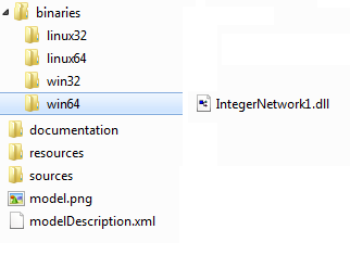
An FMU is composed of several files that will be discussed as follows:

An XML file (modelDescription.xml): This XML file contains information on the model and the definition of all variables of the FMU in a standardized way. The XML file indicates the FMI version, whether the FMU is for Model Exchange and/or for co-simulation, and the features of the FMI standard supported by the FMU. The XML file also lists the exposed model variables including inputs, outputs, states, state derivatives, and model parameters. Model parameters can be changed at the beginning of the simulation or even during the simulation for tunable parameters. Important information included in the XML is the model structural information, i.e., the variables that are output, derivatives, or unknowns at initial time. The dependency of output, derivative, and initial unknowns on other variables are also provided. This information is crucial to detect algebraic loops and correctly handle them in a model aggregated by several FMUs. The XML can also contain vendor information. It is important to indicate that information stored in the XML is not needed for execution of the model. That allows having an executable code with a minimum overhead. Below is an example of an FMI model description issued from Modelica. For more details on the XML file, refer to the section FMI description Schema in Functional Mock-up Interface for ModelExchange and Co-Simulation, Version-2.0, 2014.
```
<?xml version="1.0" encoding="UTF8"?>
<fmiModelDescription
    fmiVersion="1.0"
    modelName="ModelicaExample"
    modelIdentifier="ModelicaExample_Friction"
...
    <UnitDefinitions>
        <BaseUnit unit="rad">
            <DisplayUnitDefinition displayUnit="deg" gain="23.26"/>
        </BaseUnit>
</UnitDefinitions>
<TypeDefinitions>
    <Type name="Modelica.SIunits.AngularVelocity">
        <RealType quantity="AngularVelocity" unit="rad/s"/>
    </Type>
</TypeDefinitions>
<ModelVariables>
    <ScalarVariable
        name="inertia1.J"
        valueReference="16777217"
        description="Moment of inertia"
        variability="parameter">
        <Real declaredType="Modelica.SIunits.Torque" start="1"/>
    </ScalarVariable>
...
    </ModelVariables>
</fmiModelDescription>
```
C source file or compiled C dynamic linked libraries: These files define the model equations converted into causal form. If the source code is provided, the source code is put in the fmu://sources folder. If the model is provided in binary form, it is placed inside the folder fmu://binaries/win64. Binaries for several platforms, such as win32, linux32, and linux64, can be provided by an FMU.
Documentation (optional): Additional optional documentation can be included in the FMU inside the fmu://documentation folder.
resources (optional): Additional optional data can be included in the FMU inside the fmu://resources folder. This folder can be used for storing tables, maps or any additional data.

FMI for Model Exchange (ME)

The FMI for Model Exchange (ME) interface defines an interface to the model of a hybrid dynamic system described by differential, algebraic and discrete-time equations.

In this kind of the interface, ordinary differential equations with events and zero-crossings are handled. Algebraic equation systems might be contained inside the FMU. Also, the FMU might consist of discrete-time equations activated by events, for example a sampled-data controller. Since the overhead is small, this kind of FMU can be used for very large models as well as for small embedded systems. An FMU for Model Exchange operates in three main modes, Initialization mode, Continuous-time mode, and event-mode. The state machine of the FMU/ME is illustrated below:

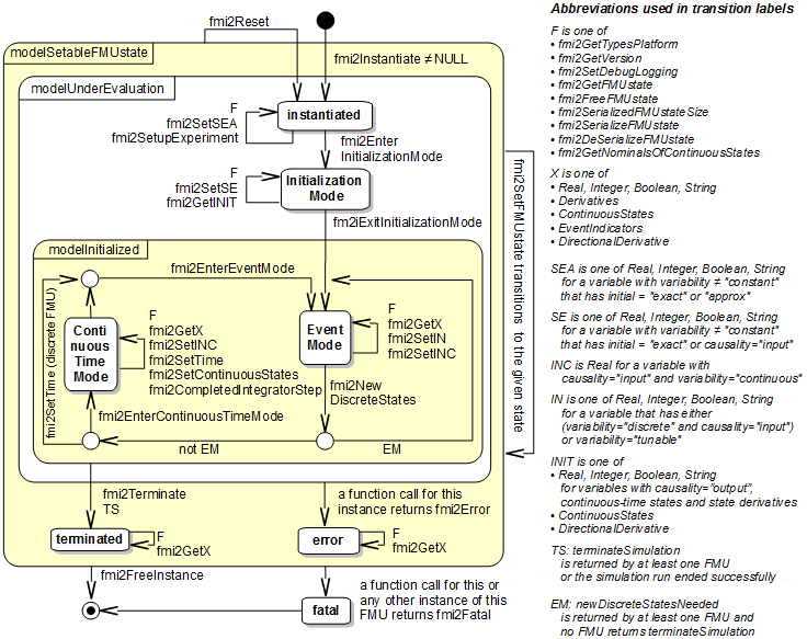
Figure 5. State Machine for FMI-2.0-Model Exchange

In initialization mode, the initial values of continuous-time states, the previous (internal) discrete-time states, are computed at the start time. In this mode, some extra equations that might not be present in other modes may be used. As an example, suppose that an FMU should start at equilibrium point. The equations defining the start value of state at equilibrium are defined only in this mode.

The continuous-time mode is used to compute the values of all continuous-time variables between events by numerically solving ordinary differential and algebraic equations. All discrete-time variables are fixed during this phase and the corresponding discrete-time equations are not evaluated.

The Event Mode is used to compute new values for all continuous-time variables, as well as for all discrete-time variables that are activated at the current event instant, given the values of the variables from the previous instant. This is performed by solving algebraic equations consisting of all continuous time and all active discrete-time equations.

The operating mode jumps from continuous-time into event-mode, if an event happens. There are four event kinds in FMI:

State-event (zero-crossing event): Event that is triggered at the time instant when the event indicator function changes from z > 0 to z ≤ 0, or vice versa. Discontinuities in a model are usually defined as zero-crossing functions (event-indicators).
Time events: Event that is triggered at a predefined time instant. Since the time instant is known in advance, the integrator can select its step size so that the event instant is directly reached. Therefore, this event can be handled efficiently.
Step-event: Event that might occur when the simulator finishes a completed integrator step. This event is not usually defined by the FMU. The simulator may use it, for example, to dynamically switch between different states, or storing data into a file.
External event: This kind of event is triggered by the environment. This event type is triggered if at the current time instant, at least one discrete-time input changes its value, a continuous-time input has a discontinuous change, or a tunable parameter changes its value.

Upon any of these events happening, the continuous-time integration is stopped and the FMU goes into the event-mode.

FMI for Co-Simulation (CS)

Co-Simulation is a general approach for the joint simulation of models developed with different tools where each tool treats one part of a modular coupled problem.

Modeling complex heterogeneous systems in engineering usually leads to hybrid systems of differential and algebraic system of equations with discrete-time equations. Such complex multi-disciplinary systems cannot often be modeled and simulated in one simulation tool alone. Sub-system models are often available only for a specific simulation tool, such as special tools for CFD (Computational Fluid Dynamics) models or integrated circuit systems. In many situations, the sub-systems is simulated with the simulator that is best suited for the specific domain. For the simulation of multi-disciplinary models, it is often reasonable or even necessary to couple different simulation tools with each other or with real world system components. Co-simulation is a general approach for the joint simulation of models developed with different tools where each tool treats one part of a modular coupled problem. The data exchange (input and output variables, status information) between sub-systems is restricted to discrete communication points. In the time between two communication points, the sub-systems are solved independently from each other by their individual solver.

Main-secondary is a common method in co-simulation. In a main-secondary approach, the secondary solvers simulate sub-models whereas the main solver is responsible for both coordinating the overall simulation and transferring data. In the main-secondary approach, instead of coupling the simulation tools directly, it is assumed that all communication (input/output data exchange) is handled via a main. Main algorithms control the data exchange between sub-systems and the synchronization of all secondary simulation solvers. Besides distribution of communication data, the main checks the connection graph, chooses a suitable simulation algorithm and controls the simulation according to that algorithm.

The secondary solvers are simulation tools, which are prepared to simulate their subtask. They are able to communicate data, execute control commands, and return status information.

FMI for co-simulation unifies the main-secondary interface and supports from simple co-simulation algorithms to more sophisticated ones. FMI provides a small set of C-functions to implement the interface. It is important to note that the main algorithm itself is not part of the standard FMI for co-simulation. The main is free to choose the appropriate co-simulation algorithm.

FMI for co-simulation supports two possible ways to provide sub-systems for co-simulation: subsystems (models) packaged along with their respective solver, which can be simulated as stand-alone components. See Figure 6.

Figure 6. Co-simulation with generated code on a single computer.

It can also be simulation as a wrapper FMU that calls its respective simulation tool to simulate the sub-system (model), which is installed externally to the FMU. See Figure 7.

Figure 7. Co-simulation with tool coupling on a single computer.

The FMI import in Twin Activate supports both implementations of FMI for co-simulation. In FMI export in Twin Activate, the solver is embedded in the FMU and no Twin Activate installation is required to run the FMU in other environments.

In FMI for co-simulation, all information relevant for the communication in the co-simulation environment is provided in the XML file. The XML file includes a set of capability flags to characterize the ability to support advanced main algorithms, e.g., the usage of variable communication step sizes, higher order signal extrapolation, or others. In Twin Activate, the simulator is considered as the main solver and each FMU block as a secondary solver.

In FMI for co-simulation, a secondary system operates in two main modes, initialization mode, and step mode. The initialization mode is used to compute the initial values for internal variables of the co-simulation secondary systems at the start time.

This mode supports a few special cases:

Some extra equation might be used that are not active during the rest of the simulation.
Algebraic equations can be solved.
If the secondary system is connected in loops with other FMUs, iterations over the FMU equations are possible.

The step mode is used to compute the values of all variables at communication points. In this mode, the main solver provides the input of secondary solvers and requests their outputs.

Co-Simulation Algorithms

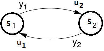
Consider a model composed of two parts (submodels) defined in two tools as shown in Figure 8.

Figure 8. Co-simulation with tool coupling on a single computer.

The outputs of submodels are computed as following equations.

\{\begin{cases} y_{1} = F_{1} (y_{2}) \\ y_{2} = F_{2} (y_{1}) \end{cases}

In order to co-simulate this system, this equation should be solved at each communication instant. F_i functions are usually complex, non-linear, and time-dependent relationships. As a result, iterative methods are the only choice for solving such equations. Three common methods used for solving them are Gauss-Seidel and Gauss-Jacobi and Newton methods. The Gauss-Seidel iteration method is represented as follows:

\begin{matrix} y_{1}^{i + 1} = F_{1} (y_{2}^{i}) \\ y_{2}^{i + 1} = F_{2} (y_{1}^{i + 1}) \\ i = 0, 1, 2, ... \end{matrix}

The Gauss-Jacobi iteration method is defined as:

\begin{matrix} y_{1}^{i + 1} = F_{1} (y_{2}^{i}) \\ y_{2}^{i + 1} = F_{2} (y_{1}^{i}) \\ i = 0, 1, 2, ... \end{matrix}

These iterative methods are simple fixed-point methods and their convergence (at most linear) depends on F_i functions. If the Fixed Point converges very slowly or diverges the Newton-type methods can be used. These methods are, however, more complicated, because in each step the Jacobian must be computed which results in higher number of simulator calls. The method which is used actually in Twin Activate is GS1, i.e., the Gauss-Seidel method with only one iteration. This method has been illustrated below:

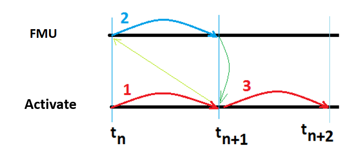
Figure 9. Co-simulation method used in Twin Activate.

The simulator of Twin Activate, which acts as the main, performs the following method for the cosimulation and synchronization between tools, as shown above.

The simulator advances the time from t_n to t_n+1, and updates the output of all blocks, except those of external tools (secondary). Optionally, the secondary system (FMU) outputs are extrapolated at a desired order if available from the FMU.
External tools are called one by one and asked to advance the their time from t_n tot_n+1 and their output is requested at t_n+1. Optionally, the secondary system (FMU) inputs are linearly interpolated.
The Twin Activate simulator takes a new step fromt_n+1 to t_n+2 using the new output value of secondary systems computed at t_n+1.
Go to step 1.

Usually, in order to get a correct result, the communication step-size (time instant between two communication instants) should not be larger than two times the highest frequency content (one-half the smallest time constant; Nyquist theorem) of the secondary systems. In practice, it should usually be smaller than this. Smaller communication step-size results in better convergence but longer simulation time. In Twin Activate, you can control the communication step-size, see the FMU block in the Block Reference Guide.

Advanced: FMI Import Preserving Full Output/Input Dependency Property

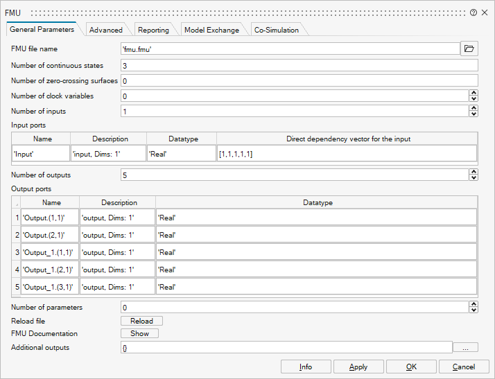
Note: This section can be skipped without losing the continuity.

A challenge in importing an FMI generated is the treatment of output/input dependencies. In a Twin Activate basic block, output and dependencies are expressed as a vector of dependencies specifying the inputs that affect any of the outputs. So the dependency is solely a property of an input port. A basic block computes all its outputs in the same call, so all its dependent inputs must be up to date when the call is made. An FMU, on the other hand, specifies output/input dependencies as a matrix specifying which output depends on each input. This input/output dependency matrix may also be different during the initialization. It provides routines that allow the computation of output ports separately and take advantage of variable caching.

A way to deal with this situation, which was the way Twin Activate imported Modelica parts, is to simply project the matrix of dependencies into a vector. This conservative approach properly assigns dependencies in Twin Activate but "loses" information along the line. This might lead in particular to detection of algebraic loops by the Twin Activate compiler that are not true algebraic loops (artificial algebraic loops). Even though there are ways to break algebraic loops in a Twin Activate model, it was decided to detect artificial algebraic loops and treat them properly. A very simple example that illustrates the problem is shown in Figure 10.

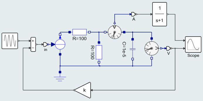
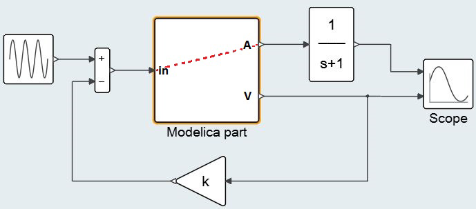
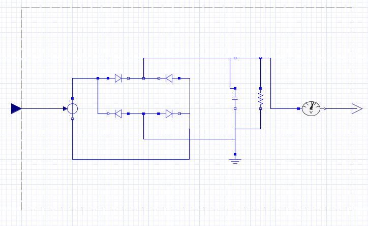
Figure 10. A simple model mixing Modelica and Twin Activate blocks.

After compiling the Modelica part, a virtual model similar to what is shown in the figure below is obtained. In the generated FMU, there is a direct dependency between the SignalCurrent input port (in) and the CurrentSensor output signal (A). The dependency is depicted by a red dashed line in Figure 11. If the dependency matrix is converted into a vector, output ports A and V depend on input port in. This direct dependency results in an artificial algebraic loop that does not really exist.

Figure 11. The model in the previous figure, after converting the Modelica part into an FMU block.

In order to solve this problem, the output/input dependency property of the basic blocks can only be set for ports separately so the imported FMU cannot be represented by a single FMU; but it can be properly represented as a network of basic blocks. The topology of this network depends on the number of inputs and outputs of the FMU and the FMUs output/input dependency matrix. A programmable super block is thus used for importing the FMU. The block main parameter is the FMU filename. By reading and parsing the XML inside the FMU, the block generates a network of basic blocks, as shown in the figure below, during the model compilation stage. The network contains a central basic block, always present, and other blocks associated with each output port. Figure 12 illustrates the resulting network for an imported FMU with two inputs and four output ports.

Figure 12. Automatically-generated Network of Basic Blocks from FMU Import for an FMU with One Input and Four Output Ports.

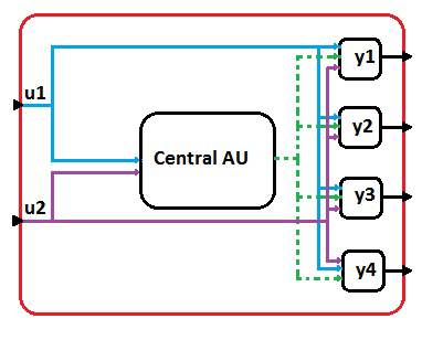
In the resulting network of basic blocks, each output unit keeps the direct-feedthrough property of the corresponding FMU output port. The central unit, on the other hand, does not have the direct feedthrough. In order to communicate within this network, the central block outputs the internal structure, which contains the FMU context, and shares it with other blocks of the network.

Note: This process is completely transparent for the user, who never sees the network in the figure above. Generating a programmable network of blocks, instead of single block for FMU import, avoids creation of artificial algebraic loops.

FMI Export in Twin Activate

Twin Activate can export super blocks as FMI-2.0 and FMI-3.0.

The FMU exported in Twin Activate is standalone, i.e., in the form depicted in Figure 6. In the FMU, the numerical solver used in the model setting is embedded in the FMU. So no Twin Activate installation is required to run the FMU in other environments.

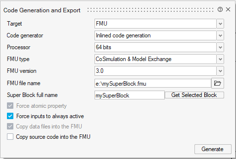
In order to export a model or a part of a model, the interested region should first be placed into a super block. After it is converted into a super block, right-click on the Code Generation and Export menu. The Code Generation dialog is opened, as shown in Fig.12.24.

Figure 13. A Bridge Rectifier Modeled in MapleSim.

Figure 14. Simulation Result of Model in Previous Figure in MapleSim.

By selecting FMU as target, two export methods will be available:

Standard Code Generation: In this method, the same libraries used in Twin Activate will be packaged inside the FMU. This method supports more Twin Activate blocks for FMU export, but since all necessary libraries binaries are included in the FMU, the FMU size may be big.
Inline Code Generator: In this method, an optimized C code is generated for Twin Activate block. The generated C code can be exported in the FMU and recompiled for another OS.
Note: Note that Modelica blocks can be exported in standard code generation, as well as in inlined code generation for Co-Simulation.
Note: Some Twin Activate blocks, such as Modelica blocks, cannot be exported with inlined code generation for Model Exchange.
Note: Inlined code generation also can export as FMI-3.0 and supports arrays and clocks.

The name and identifier of the exported FMU will be the name of the super block. Hence, if the name of the super block contains unsupported characters, they are converted to "_". For example if the name of the super blocks is SuperB !%lock, sb_SuperB___lock will be used instead.

Figure 15. FMI Block Dialog in Twin Activate

In the Code Generation and Export dialog, the super block can be exported with Model Exchange and/or Co-simulation interface types. If the super block is exported as FMI for co-simulation, the Twin Activate simulator as well as the simulation parameter values in the setup menu will be used in the exported model. If a model is implicit, i.e., contains implicit blocks, such as ImplicitDerivative, Constraint, or Automaton, it can only be exported as FMU for Co-Simulation. In this case, an implicit solver such as, Ida, Daskr, or Radau(DAE) is used inside the FMU.

Nested FMU

A super block containing other FMUs (FMI-1.0 or FMI-2.0 of type Model Exchange or co-simulation) can be exported as a new FMU.

Figure 18. Code Generation and Export Dialog in Twin Activate

Exporting Modelica

A super block containing Modelica components can be exported as FMU.

Note: The super block cannot have Modelica ports (implicit Twin Activate ports).

All input and output ports should be of explicit signal type to be exported as FMU. Note that Modelica blocks can be exported in Standard code generation for FMU export, as well as in Inline code generator for Co-simulation. Inlined code generation does not support FMI Export with Model Exchange interface type for Modelica blocks.

Shortcomings

The current version of the FMI export of Twin Activate does not support the following features:

Signal import blocks FromBase and SignalIn are not supported.
Signal export blocks ToBase and SignalOut are not supported.
Signal Viewer blocks such as Scope, Display, etc. are ignored.
Co-simulation blocks such as MotionSolve or Flux blocks are not supported.
Memory block is not supported.

Requirements

The FMI export facility needs a Microsoft Visual Studio C++ compiler installed on the system. Otherwise, the generated C code cannot be compiled and no binary will be available for the FMU and FMI export fails. Twin Activate automatically detects the C compiler on the system. In order to detect the C compiler, you may use the command: vssGetCompilerName().

Note: The tcc compiler cannot be used in FMI export.

Example

In order to demonstrate the way a model in Twin Activate can be exported, here is an example. Open the model Controller_Me_CS.scm available in the product installation directory, under tutorial_ models/Extended_Book_Models/Chapter_11_FMI folder. Suppose that we want to export the indicated region in the model, as shown in Figure 19

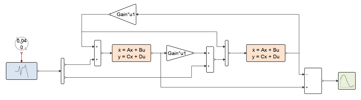
Figure 19. Controller Model (AFM_controller.scm).

Select the region and convert it into a super block as shown in Figure 20 Rename the super block as needed to the name of the FMU to be generated.
Figure 20. Controller Model after Super Block Creation (SFM_controller.scm).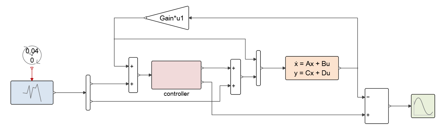
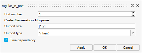
If the super block contains input ports, inside the super block, click on the Input blocks and select the Time dependency check box and fill the input dimensions with the correct values, as shown in Figure 21. Otherwise, an FMU with only discrete-time variables will be generated and the size of input ports will be one.
Exit the super block and, select the super block, and open Export > Export from the ribbon.
Select the export type: Model Export, Co-Simulation, or both.
The C code and the binaries are generated in the Twin Activate model temporary folder.
After the FMU is generated, a dialog opens. Select a folder to copy the FMU into.

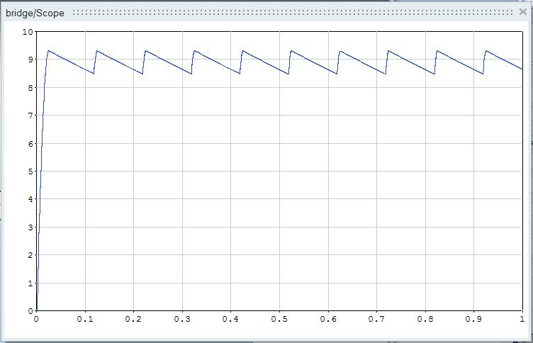
The generated FMU can be imported as an FMU with the FMU block and be tested to verify whether it gives the same result.

Advanced User Topics

The co-simulation algorithm is not a part of the FMI standard and tools are free to choose the best method to perform the co-simulation with an FMU. The FMI import block is basically a Twin Activate block that interfaces an FMU (Model Exchange or Co-Simulation) with Twin Activate. Similar to any other Twin Activate block, the FMI import block is called with several flags during the simulation. The model is updated through the propagation of block outputs throughout the whole model. In the output propagation, the input/output dependency of the blocks plays an important role. For example, if at least one output of a block depends directly on the i^th input of the block, the block is not called (i.e., its outputs are not updated) unless i^th input is updated. This is guaranteed by the Twin Activate compiler to ensure that at any time instant and for a given continuous-time state, the outputs are correctly evaluated. After all input and outputs are evaluated, other jobs, like reading derivative of continuous-time states, evaluating the zero-crossing surfaces, programming a discrete event, or in the case of co-simulation with an FMU calling fmixDoStep can be done. For more details about the simulation flags and calling blocks the reader is referred to in the "Twin Activate blocks" chapter of the Extended Definitions PDF.

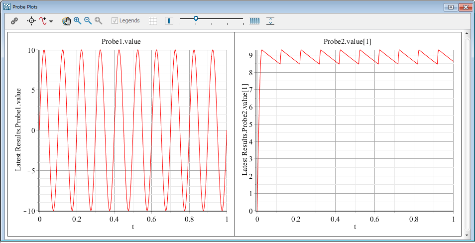
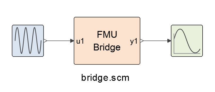
For the sake of simplicity, consider a Twin Activate model containing only one FMU, as shown in Figure 22. The FMU has only one input and one output port. The whole Twin Activate part is abstracted into a single block. In co-simulation, the standard part of the Twin Activate model and the FMU exchange their input and output signals at some time instants called communication points (CP). Between two subsequent CPs Twin Activate simulator engine and FMU simulate separately with their respective solver. At the communication step t_i, the Twin Activate simulator engine takes the lead and performs the simulation until the next communication step, i.e., simulate the interval [t_i, t_i+1]. During the integration between t_i and t_i+1, the outputs of the FMU can be extrapolated. Mathematically speaking, the Twin Activate simulator engine performs the simulation of this model for the interval t_i ≤ t ≤ t_i+1, where x_A is Twin Activate continuous-time states and u_A is the input of the Twin Activate part. y_F , y′_F and y′′_F are output of the FMU block, and their first and second time derivatives, respectively. If extrapolation is disabled (i.e., zero order extrapolation method is selected) then $u_{A} (t) = y_{F} (t_{i})$ .

\{\begin{matrix} {\dot{x}}_{A} = f (x_{A}, u_{A} (t)) \\ u_{A} (t) = y_{F} (t_{i}) + (t - t_{i}) {y^{'}}_{F} (t_{i}) + \frac{{(t - t_{i})}^{2}}{2} y_{F}^{n} (t_{i}) + ... \end{matrix}

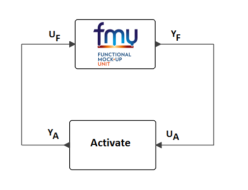
During the integration of the Twin Activate part, the FMU may be invoked several times to retrieve y_F(t_i), y′_F(t_i), y′′_F(t_i), etc.

After the Twin Activate engine simulates the interval [t_i, t_i+1], and y_F(t_i+1) is evaluated, it is the FMU's turn to advance and simulate the same interval. Right before invoking fmixDoStep, the input values of the FMU at t_i (i.e., u_F(t_i) and possibly its first order derivative ( i.e., der(U_F(t_i))) are given to FMU (using fmi2SetXXX and fmi2SetRealInputDerivatives commands). Also, the value of u_F(t_i+1 is read and saved for subsequent fmixDoStep calls.

The derivative of input is computed as follows:

d e r (U_{F} (t_{i})) = \frac{u_{F} (t_{i + 1}) - u_{F} (t_{i})}{t_{i + 1} - t_{i}}

After FMU inputs are set, the FMU is called to perform fmixDoStep(cp=t_i, h=t_i+1 − t_i).

Controlling the Co-Simulation Communication Step

In the co-simulation with an FMU, the size of communication steps is governed by the numerical solver of Twin Activate (see the model settings panel). If a variable step-solver is chosen, the communication step will be variable and with a fixed-step solver, the communication steps will be fixed. In some cases, this behavior is not desired. Consider, for example, a complex Twin Activate model where a variable step-solver is needed but calling fmixDoStep in an FMU is costly. In this case, the user has the possibility of choosing a fixed-communication step size in the FMU parameter settings (see the FMU block in the Block Reference Guide) .

Unlike the variable communication step size where every Twin Activate numerical solver step is followed by a fmixDoStep in the FMU, if a fixed-Communication step is chosen by the user, fmixDoStep is called periodically, regardless of Twin Activate Solver steps. Upon dependence of the output of the FMI block on the rest of the model, Twin Activate solver meshpoint may or may not coincide with the communication points of FMI. For example, if the output of the FMI block does not go to any block with continuous-time state, the solver mesh-point and communication points do not coincide.

Calling fmixDoStep

As described in Co-Simulation Algorithms, Twin Activate and the FMU for co-simulation alternate between calling their respective solvers to solve and advance time between communication points and coupling shared data (inputs/outputs) at these communication points. At any particular time (t_i), Twin Activate will take a time step from t_i to t_i+1 first and then call to the FMU to advance the time with fmixDoStep. Twin Activate calls fmixDoStep for either the flag VssFlag_OutputUpdate or VssFlag_EventScheduling depending on the model and FMU parameter settings.

Blocks in Twin Activate are called in a predefined order with flag VssFlag_OutputUpdate, in order to read the output ports. The simulator propagates the updated output port values all over the model. After all input and output ports of blocks are updated, the blocks can be called (maybe in an arbitrary order) to do the update job with flag VssFlag_EventScheduling and VssFlag_StateUpdate (see section "Simulation function implementation" of the "Twin Activate blocks" chapter in the Extended Definitions PDF for more details).

In one case for calling DoStep in FMU for co-simulation blocks, after the input/output update phase at t_i+1, the input value of the FMU block at t_i (and possibly their derivatives) are given to the FMU. Then fmixDoStep is called in flag VssFlag_EventScheduling to advance the FMU time from t_i to t_i+1. The flags and the job that the block should do in each flag has been explained in chapter 9 of the Extended Definitions PDF.

It is important to note that if fmixDoStep is called in flag VssFlag_EventScheduling, the output of the FMU are not immediately read because this is the purpose of the flag VssFlag_OutputUpdate, which was called prior to VssFlag_EventScheduling. The outputs of the FMU will be updated in the next model input/output update with flag VssFlag_OutputUpdate.

This usually introduces a communication step delay in the output signal versus the input signal. In some situations, it is possible to perform fmixDoStep during the input/output update phase, i.e., with flag VssFlag_OutputUpdate. In this case, the newly updated output can be propagated through the model and the delay be avoided. The situations where fmixDoStep will be called in flag VssFlag_OutputUpdate are:

If the FMU block does not have any input port, no need to wait all input/output update propagation to call fmixDoStep. At the block invocation to retrieve u_A(t_i+1) (which is equal to y_F(t_i)), fmixDoStep will be called and immediately y_F(t_i+1) can be obtained and propagated into the model. In this way, the delay is avoided.
If the variability of all inputs is discrete or none of input data-types is Real, u_F(t) will be equal to u_F(t_i) all over the interval [t_i, t_i+1]). As a result, fmixDoStep will be called at input/output update with flag VssFlag_OutputUpdate.
If the input interpolation is off or the FMU does not support interpolation, u_F(t) will be equal to u_F(t_i) all over the interval [t_i, t_i+1]). As a result, fmixDoStep will be called at input/output update with flag VssFlag_OutputUpdate.
After all input values of FMU at t_i+1 are read during the input/output update phase with flag VssFlag_OutputUpdate. As an example, consider the case where an output of the FMU depends directly on all input ports of the FMU. After the value of the output port is requested by the simulator, it means that all inputs are already updated by the simulator at t_i+1. As a result, fmixDoStep can be immediately called and the FMU output y_F(t_i+1) can be propagated for the FMU outputs whose value are not already propagated.

Input Interpolation and Output Extrapolation in Co-Simulation

Twin Activate is a hybrid simulation tool which means it can simulate a model with continuous-time and discrete-time parts. The discrete-time part is activated by discrete-time events and the continuous-time part of the model is integrated by the numerical solvers of Twin Activate. Discrete-time events cause discontinuities in signals. As a result, signals in a hybrid model may be piece-wise continuous. Since several discrete-time events may happen at the same time, a signal may have several values at the same time instants, as shown in Figure 23.

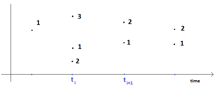
Figure 23. Evaluation of a Model at Different Time Instants

The multiple time instants at an event time is also called super dense time instants. During the integration of the continuous-time part, the numerical solver takes steps to advance the time. At the beginning of each step, the time dependent part of the model are evaluated with the flags VssFlag_OutputUpdate, VssFlag_EventScheduling, and VssFlag_StateUpdate. The time instant where the model is evaluated at the beginning of the solver step is also called a solver mesh-points. Discrete-time events are classified in two categories, critical and non-critical events. Critical events are discrete-time events that may cause discontinuities in the continuous-time part of the model. If a critical event happens, the numerical solver needs to be cold-restarted. For more details about events and solvers, refer to the chapter on "Twin Activate hybrid simulator and its interface with numerical solvers" in Extended Definitions PDF. Following one or several critical events, there is always a solver mesh-point to update the continuous-time parts. In other words, after the evaluation of a model at critical events, the continuous-time part should be evaluated before starting the integration of the continuous-time part. Unlike critical events, after a non-critical events, there is not necessarily a mesh-point. Non-critical events may happen between two mesh-points.

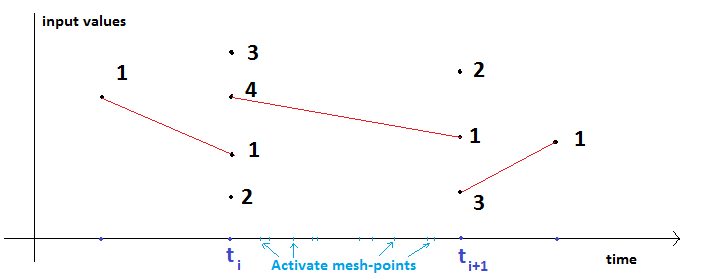
If the Preferred fixed communication stepsize in the Co-Simulation tab of the FMU block, is left zero, then the Twin Activate solver mesh-points are taken as the co-simulation communication points, i.e., in Fig.12.30 t_i and t_i+1 are Twin Activate mesh-points and also communication points. Since the model may have critical events, the model may get evaluated several times at communication instants. Before calling fmixDoStep at the mesh-point t_i+1, the input of the FMU at the mesh-point (i.e., u_F(t_i)) is given to the FMU. If the derivative of the input is also provided to the FMU, Twin Activate computes the first order derivative of the input by using the following equation:

d e r (U_{F} (t_{i})) = \frac{u_{F} (t_{i + 1}) - u_{F} (t_{i})}{t_{i + 1} - t_{i}}

Note: In order to compute the derivative of the input, the input value at the mesh-point evaluation, as well as the first super dense time at the next communication points is used, see Figure 24.

Figure 24. First-Order Interpolation of FMU Inputs in Presence of Events at Communication Steps.

If the Preferred fixed communication stepsize in the co-simulation tab of the FMU block is non-zero, then the communication points are periodic. i.e., in Figure 25, t_i and t_i+1 are communication points. Between communication points, there may be several Twin Activate mesh-points, see Figure 25. The FMU is activated by a periodic events where at each event time, fmixDoStep is called. In this case, before calling fmixDoStep at the event time of t_i+1, the input of the FMU at the previous communication point (i.e., u_F(t_i)) is given to the FMU.

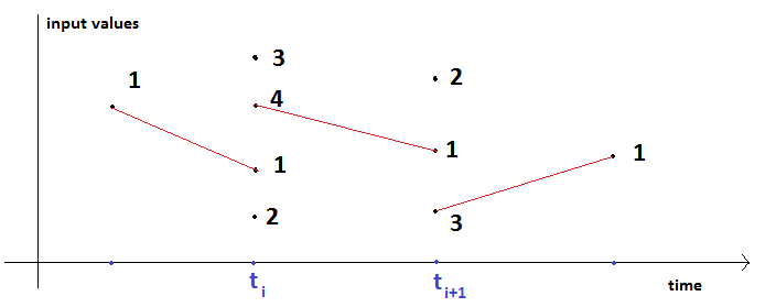
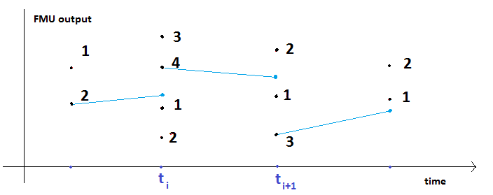
Figure 25. First-Order Interpolation of FMU Inputs in Presence of Events at Communication Steps (Fixed Communication Step).

Based on FMU attributes, Twin Activate chooses to call fmixDoStep at t_i+1 either during the call with flag VssFlag_OutputUpdate, or during the call with flag VssFlag_EventScheduling. When the Twin Activate solver integrates the interval [t_i, t_i+1], the output of the FMU block is computed with the following formula (if a linear output extrapolation is used).

y_{F} (t) = y_{F} (t_{i}) + (t - t_{i}) {y^{'}}_{F} (t_{i})

At t_i+1, the output of FMU is $y_{F} (t_{i + 1}^{1}) = y_{F} (t_{i}) + (t_{i + 1} - t_{i}) {y^{'}}_{F} (t_{i})$ until fmixDoStep is called at the mesh-point and the output of FMU is retrieved. The output is retried and displayed at the next communication point.

Figure 26. First-Order Extrapolation of FMU Output in Presence of Events at Communication Steps.

References

Functional Mock-up Interface for Model Exchange. Version-1.0, 2010.
Functional Mock-up Interface for Co-Simulation. Version-1.0, October 2010.
Functional Mock-up Interface for ModelExchange and Co-Simulation, Version-2.0, 2014.