Test Case A
This example describesthe calculation ofthepoyting vector andthe maximum value of the field on an observationplaneofpointsnear the antenna.By calculating themultipolein this firstsimulation,thencalculatethe same dataonother observation, this timecylindrical,around yhe antenna and usingthe multipolefor a gainintime.
Step 1: Create a new MOM Project.
Open 'New Fasant' and select 'File --> New' option.
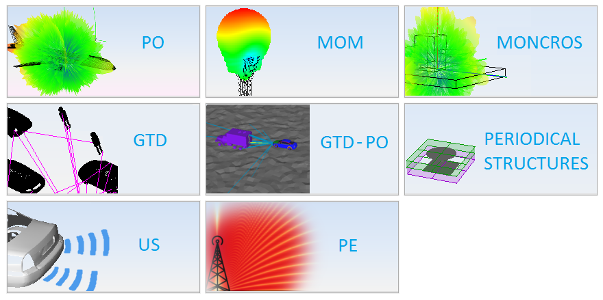
Select 'MOM' option on the previous figure and start to configure the project.
Step 2: Create the geometry model.
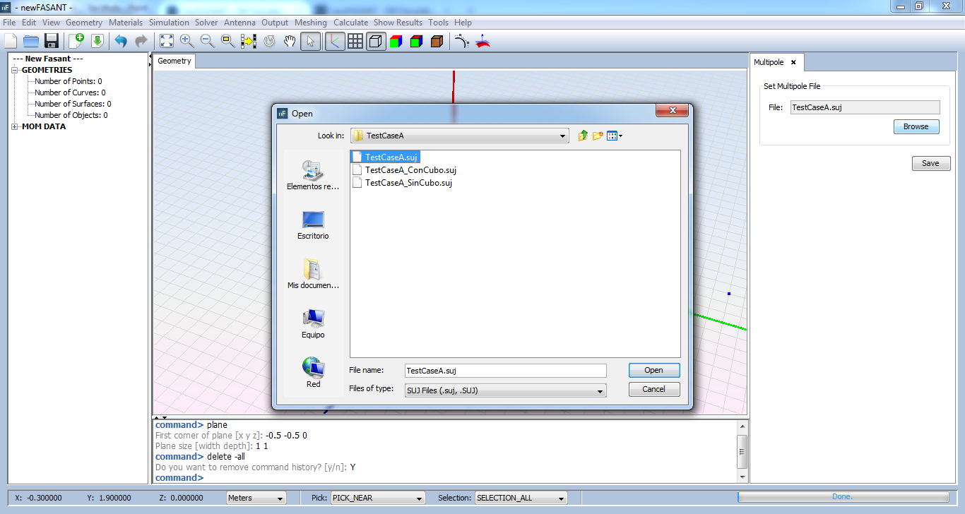
Execute 'plane' command writing it on command line and sets the parameters as the next figure shows when command line ask for it.

Step 3: Set Simulation Parameters
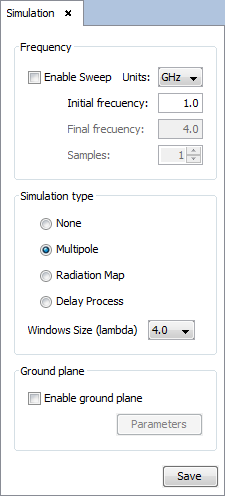
Select 'Simulation --> Parameters' option on the menu bar and the following panel appears. Set the parameters as the next figure shows and save it.
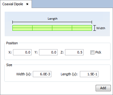
Step 4: Set the antenna parameters.
Select 'Antenna --> Primitives --> Coaxial Feed --> Dipole' option and set the parameters as show the next figure. Then save the parameters and the antenna appears.
Step 5: Set Near Field parameters.
Select 'Output --> Observation Points' option. The following panel will appear.
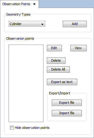
To add a plane visualization, select 'plane' on the selector of 'Geometry Types' section and click on 'Add' button. The plane parameters panel will appear, then configure the values as the next figure show and accept it clicking on 'OK' button.
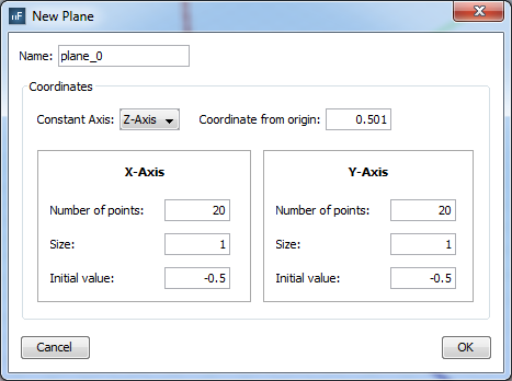
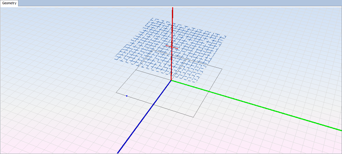
The observation will appear as a dashed line on the position configured.
Step 6: Meshing the geometry model.
Select 'Meshing --> Parameters' to open the meshing configuration panel and then set the parameters as show the next figure.
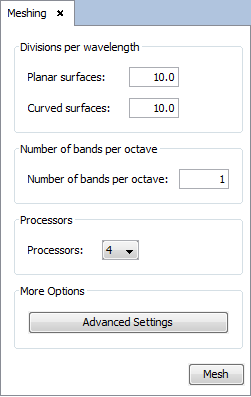
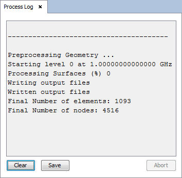
Then click on 'Mesh' button to starting the meshing. A panel appears to display meshing process information.
Step 7: Execute the simulation.
Select 'Calculate --> Execute' option to open simulation parameters. Then select the number of processors as the next figure show.
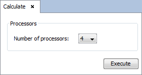
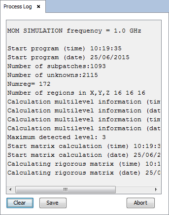
Then click on 'Execute' button to starting the simulation. A panel appears to display execute process information.
Step 8: Show Results
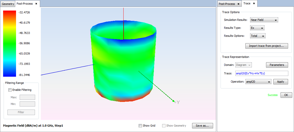
Select 'Show Results --> Post-Process' option to calculate the puyting vector of the observation. To see the result as a diagram, select 'diagram' on the selector of 'New Trace' option and click on 'OK' button.
Then, a panel to configure the results appears. Set the parameters as next figure and add on 'OK' button.
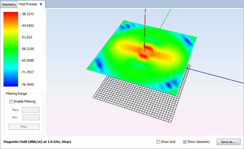
The visualization of the results appears on the main panel.
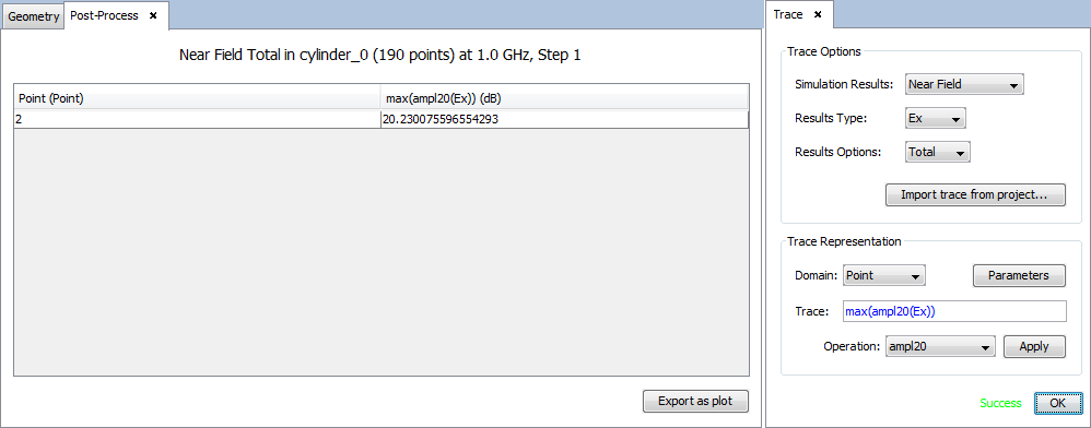
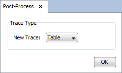
Select 'Show Results --> Post-Process' option to calculate the maximum field value of the plane observation. To see the result as a table, select 'table' on the selector of 'New Trace' option and click on 'OK' button.

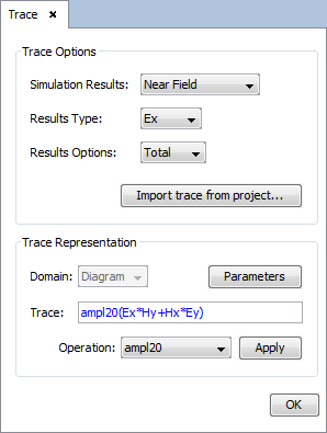
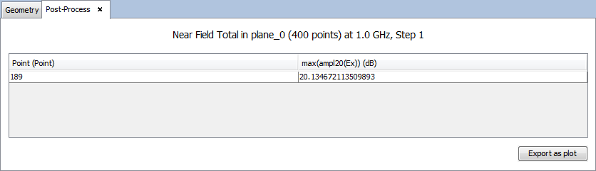
Then, a panel to configure the results appears. Set the parameters as next figure and add on 'OK' button.
Step 9: Save the multipole file to use it for calculating the second observation.
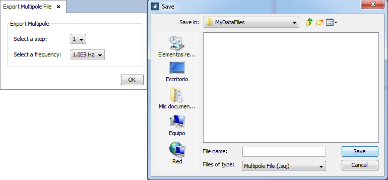
Select 'Show Results --> Export Multipole File' option to save the multipole file on a selected path for use on other simulations. Previous, select the step and frequency for the multipole file.
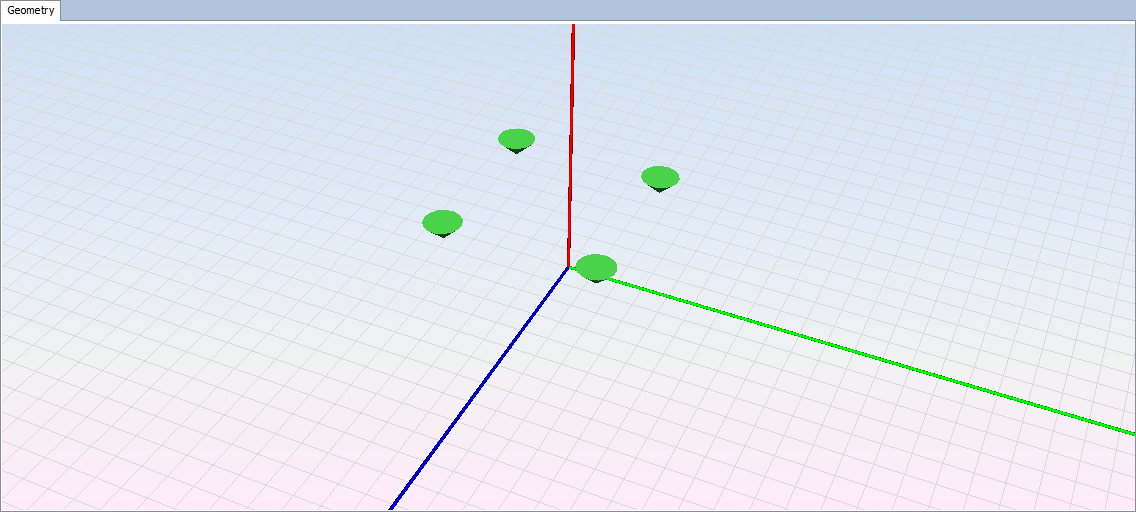
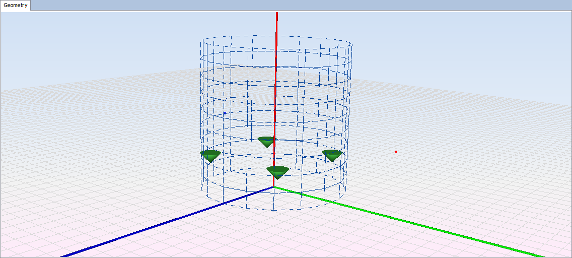
Step 10: Delete the geometry model, the antena and the observation plane. Then set the multipole file saved as antenna selecting 'Antenna --> Multipole Antenna' option and selecting the '.suj' file saved en the step 9. Then click on 'Save' button and the multipole appears as green cone.
Step 11: Set Near Field parameters.
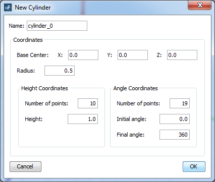
Select 'Output --> Observation Points' option. To add a cylindrical visualization, select 'cylinder' on the selector of 'Geometry Types' section and click on 'Add' button. The cylinder parameters panel will appear, then configure the values as the next figure show and accept it clicking on 'OK' button.
The observation will appear as a dashed line on the position configured.
Step 12: Calculate again (meshing is not necessary and not work without a geometry). This calculation uses the multipole antenna as the geometry and the coaxial dipole used in the first simulation.
Step 13: Show results again like step 8.