Example 2: Dynamic Simulation

In this section, we will explain how to compute the Near Field of a dynamic simulation using a simple geometry.

Step 1: Create a newFASANT project for running a GTD simulation. To do this, select the File → New option (or press Ctrl+N) and press the following icon in the panel that appears in order to create a GTD project:

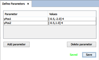
Step 2: Since we want a dynamic simulation, we need to define some parameters in order to be able to parametrize our geometry. In this simulation, we will create two boxes moving in opposite directions along the Y axis. These boxes will move at a rate of 0.5 meters per step, considering a total of 4 steps. To add a parameter, select the Geometry → Parameters → Define Parameters option and press the Add parameter. A new row in the parameters table will be created. Change the name of the parameter to something more descriptive like “yPos1” and change the text in the Values column to:

[-0.5, -2.0] 4

This can be read as “This parameter will take four equally spaced values, beginning in-0.5 and ending in -2.0” (so the parameter will take the values -0.5, -1.0, -1.5 and -2.0).

Repeat the same procedure to add a new parameter called “yPos2”, which will describe the movement of the second box. Set the content of the Values column of this second parameter to the following text:

[-0.5, 1.0] 4

Press the Save button to save the parameter settings.

Step 3: Now we will create the geometry for the simulation. Let’s create both boxes using the command line (the command line is the panel at the bottom side of the window, below the geometry view). The following figure shows the commands to be entered into the command line in order to create the boxes.

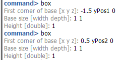
As we can see, we have used the parameters created in the previous step to define a varying Y coordinate in the boxes. The result is shown in the following figure. Note that the following figure depicts the state of the geometry in the first step (i.e. both parameters are equal to the first value in their set of values):

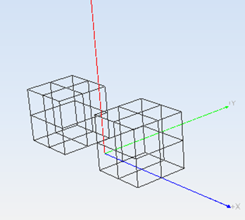
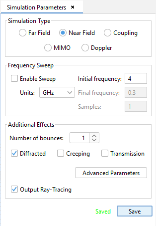
Step 4: Now we are going to set up the parameters of the simulation. Select Simulation Parameters → Simulation. Enter the following parameters:

• Near Fieldsimulation type.
• Initial frequency 4.0 GHz.
• Disable Frequency Sweep.
• Enable diffraction.
• Keep the number of bounces equal to 1.

Step 5: Define an antenna over the cube by selecting the option Antennas → Dipole Antenna and setting up the antenna parameters as in the following figure:

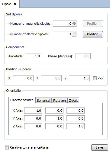
Press the Add button to add the antenna to the simulation.

Step 6: Now we are going to add a line of observation points. Select the Output → Observation Points option. In the Geometry Types combo box, select Line and press the Add button. The following dialog will pop up. Set the line parameters as shown in the figure.

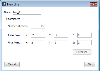
Press OK button to add the observation line.

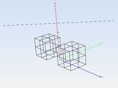
Step 7: Select Meshing → Create Visibility Matrix to mesh. Select the number of processors to use for the meshing process and press the Mesh button.

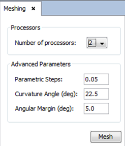
Step 8: Once the meshing process has finished (no more text is being outputted into the process log), we are ready to run the simulation. To do this, select Calculate → Execute, select the number of processors to use (like we did before meshing) and press the Execute button.

Step 9: When the calculation has finished, press Show Results → View Ray. In the left side of the Ray Visualization panel, select Step 2. The result should be the same as in the following figure:

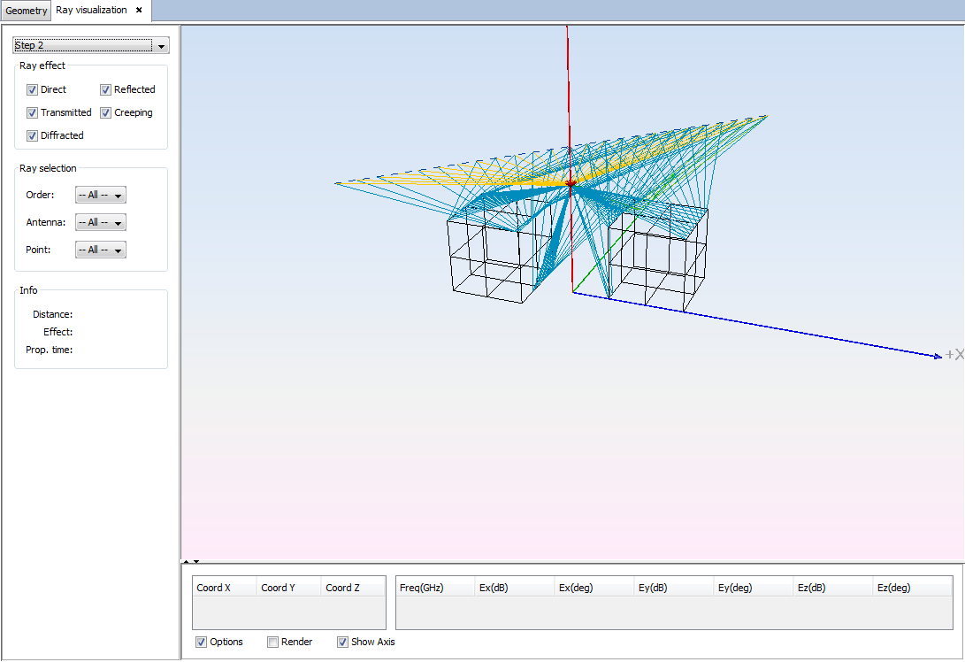
Step 10: It is possible to select a ray to show its information. Clicking in one of the rays will fill its information in the bottom of the panel.

Step 11: To visualize the angular cuts, click on Show Results → Near Field → View Cuts.

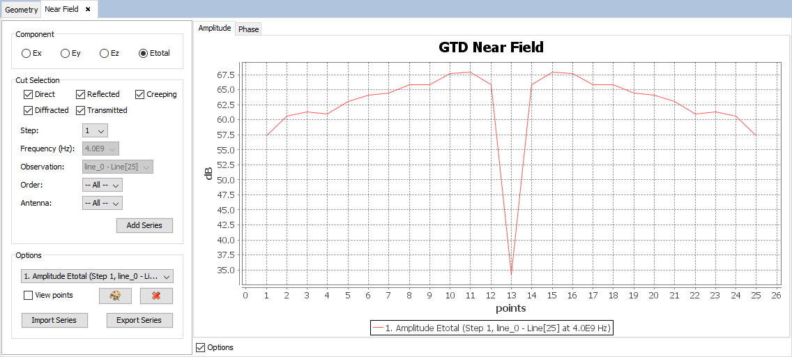
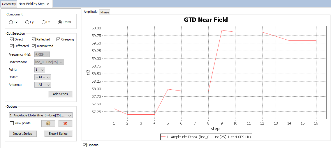
Step 12: To visualize the evolution of the near field along the different steps of the simulation, select Show Results → Near Field → View Cuts by Step: