OS-HM-T: 1010 Linear Static Analysis with Thermal Loading of a Coffee Pot Lid
Tutorial Level: Beginner In this tutorial, an existing finite element model of a plastic coffee pot lid is used to
demonstrate how to apply thermal loading and perform an OptiStruct linear static analysis.
Before you begin, copy the file(s) used in this tutorial to your
working directory.
HyperView post-processing tools are used to determine
deformation and stress characteristics of the lid.
The following exercises are included:
Retrieve the HyperMesh database file.
Set up the problem in HyperMesh.
Apply loads to the model.
Submit the job.
View the results in HyperView.
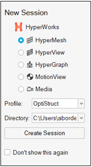
Launch HyperMesh
Launch HyperMesh.
In the New Session window, select HyperMesh from the list of tools.
For Profile, select OptiStruct.
Click Create Session.
Figure 1. Create New Session This loads the user profile, including the appropriate template, menus,
and functionalities of HyperMesh relevant for
generating models for OptiStruct.
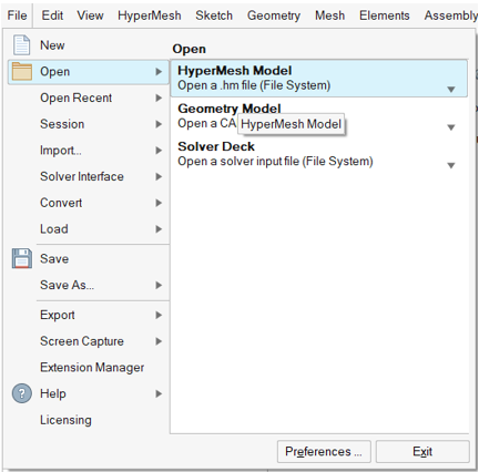
Open the Model File
On the menu bar, select File > Open > HyperMesh Model.
Navigate to and select the coffee_lid.hm file saved in your
working directory.
Click Open.
The coffee_lid.hm database is loaded into the current
HyperMesh session, replacing any existing
data.Figure 2. Model Import Options
Tip: Alternatively, you can drag and drop the file onto the
viewport from the file browser window.
The database
contains meshed data, contact definitions, and control
cards.
Set Up the Model
The outline of the fatigue analysis setup in this tutorial is shown
in the block diagram.Figure 3. Fatigue Setup Sine Sweep - SN Damage
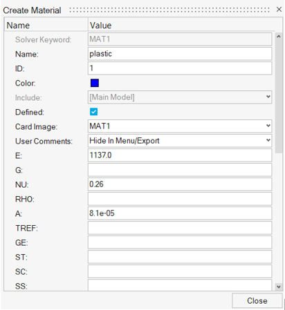
Create the Material
The imported model has two component collectors with no materials. A material
collector needs to be created and assigned to the component collectors.
In the Model Browser, right-click and select
Create > Material.
A default MAT1 material template displays in the
Entity Editor.
For Name, enter plastic.
Enter the following material values in the dialog:
[E] Young’s modulus = 1137
[NU] Poisson’s ratio = 0.26
[A] Coefficient of linear thermal expansion =
8.1e-05
The material uses the OptiStruct linear isotropic
material model, MAT1. If a material property does not
display a value next to it, it is turned off. It is not necessary to define a
density value since only a static analysis is performed. Density values may be
required for other solution sequences.Figure 4. Material Property Values for plastic
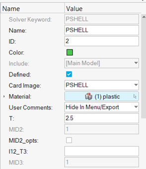
Edit the Properties and Update the Component Collector
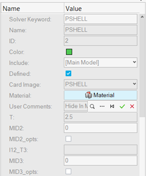
In the Model Browser, expand the
Property folder and click on
PSHELL.
The PSHELL property entry is displayed in the Entity
Editor.
Verify the thickness value, T, is set to 2.5.
Notice the value field for Material is set to <Unspecified>.
This indicates that no material properties are being referenced by this
property.
For Material, select Unspecified > Material.
Figure 5. Select the Material plastic for the Property
PSHELL
In the Select Material dialog, select
plastic and click OK.
The material, plastic, is now assigned to the property
PSHELL. Figure 6. PSHELL Property Entry Fields in Entity Editor
Repeat steps 1 through 5 to assign the plastic property to
PSHELL1.
Apply Loads to the Model
Constraints have already been applied to the model. In the following steps, thermal
loading is applied.
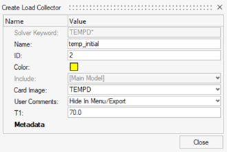
Create a Load Collector
In the Model Browser, right-click and select
Create > Load Collector.
A default load collector template displays in the Entity
Editor.
For Name, enter temp_initial.
For Card Image, select TEMPD.
For Default Temperature Value (T1), enter 70.
Click
Close.
Figure 7. Create temp_initial Load Collector
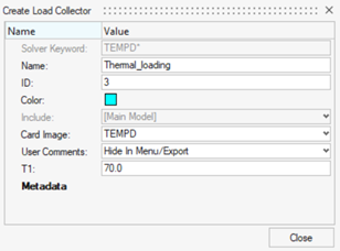
Similarly, create another load collector with the name
thermal_loading.
For Card Image, use TEMPD.
For Default Temperature Value (T1), enter 70.
Click
Close.
Figure 8. Create thermal_loading Load Collector
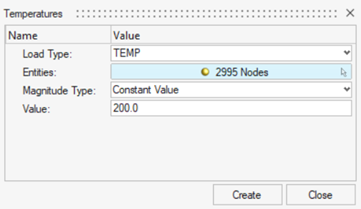
Create a Temperature Load
From the Analyze ribbon, select Temperatures.
For Entities, choose Nodes.
From the Advanced Selection window, select both
PSHELL and PSHELL1, then click
OK.
For Value, enter 200.
Click Create and Close.
Figure 9. Create Temperature Load
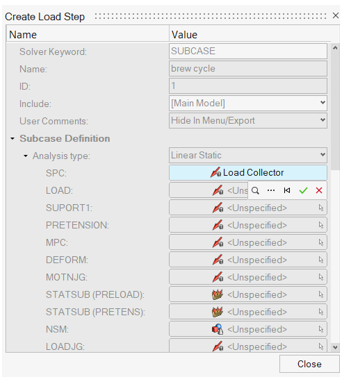
Create a Subcase
OptiStruct subcases are also referred to as load
steps.
In the Model Browser, right-click and select
Create > Load Step.
A default load step template displays in the Entity Editor.
For Name, enter brew cycle.
For Analysis type, select Linear Static.
For SPC, select Unspecified > Loadcol.
Figure 10. Select Constraints
In the Select Loadcol dialog, select
constraints and click
OK.
Select the TEMP check box.
For TEMP, click Unspecified > Loadcol.
In the Select Loadcol dialog, select
temp_initial and click
OK.
Similarly, select the TEMP_LOAD and for TEMP_LOAD,
select Unspecified > Loadcol.
In the Select Loadcol dialog, select
THERMAL_LOADING and click
Close.
Figure 11. Create brew cycle Load Step
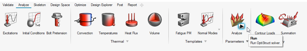
Submit the Job
Run OptiStruct.
From the Analyze ribbon, click Run OptiStruct
Solver.
Figure 12. Select Run OptiStruct Solver
Select the directory where you want to write the OptiStruct model file.
For File name, enter lid_complete.
The .fem filename extension is the recommended extension
for Bulk Data Format input decks.
Click Save.
Click Export.
For export options, toggle all.
For run options, toggle analysisoptimization.
For memory options, toggle memory default.
Click Export.
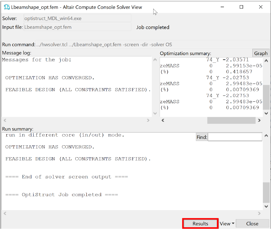
The .fem file is exported. The Compute Console
should open with the file loaded in Input file(s).
In the Altair Compute Console, click
Run.
If the job is successful, an "OptiStruct Job Completed" message appears
in the Compute Console Solver View Message Log. New results
files are in the directory where the model file was written. The
lid_complete.out file is a good
place to look for error messages that could help debug the input deck if any
errors are present.
The default files written to your
directory are:
lid_complete.html
HTML report of the analysis,
providing a summary of the problem formulation and the analysis
results.
lid_complete.out
OptiStruct output file containing
specific information on the file setup, the setup of your
optimization problem, estimates for the amount of RAM and disk
space required for the run, information for each of the
optimization iterations, and compute time information. Review
this file for warnings and errors.
lid_complete.h3d
HyperView compressed binary results
file.
lid_complete.stat
Summary of analysis process, providing CPU information for each
step during process.
Figure 13. Run Summary
View Contour Plot of Stresses and Displacements
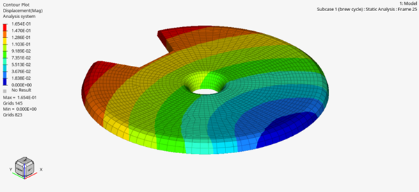
Click Contour.
For Results type, select Displacement (v).
For Data type, select Mag.
This represents the magnitude of the displacements.
Click Apply.
A contoured image of your model should be visible. The contours
represent the displacement field resulting from the applied loads and boundary
conditions.Figure 14. Contour Plot Showing Displacement
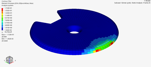
For Results type, select Element Stresses (2D &
3D).
For Data type, select von Mises.
Click Apply.
Each element in the model is assigned a legend color, indicating the von
Mises stress value for that element, resulting from the applied loads and
boundary conditions.Figure 15. Contour Plot Showing von Mises Element Stress