OS-HM-T: 2000 Direct Transient Analysis of Airframe Model
Tutorial Level: Beginner This tutorial demonstrates how to perform direct transient dynamic analysis using OptiStruct using an existing finite element model of a wing
structure. HyperView is used to post-process the deformation
characteristics of the Wing Structure under the transient dynamic loads.
Before you begin, copy the file(s) used in this tutorial to your
working directory.
Figure 1. Finite Element Model of Wing Structure Airframe Model
The wing structure is constrained in all the DoFs at the bolt joints by using rigid
elements represented by the rigid2 component. Transient dynamic pressure load is
applied at the grid points in in the negative z-direction. The time history of the
loading is shown in the next figure. The direct transient analysis is run for a
total time of 3 seconds with the time divided into 30 increments (meaning the time
step is 0.1).
Figure 2. Time History of Applied Pressure Loading
The following exercises are included:
Create the time-dependent dynamic pressure load or the variation of load
versus time
Create the time step for transient analysis
Create the direct transient subcase to include the load collectors
Run a direct transient dynamic analysis
Post-process the results using HyperView
Launch HyperMesh
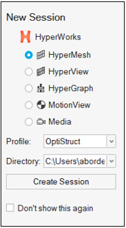
Launch HyperMesh.
In the New Session window, select HyperMesh from the list of tools.
For Profile, select OptiStruct.
Click Create Session.
Figure 3. Create New Session This loads the user profile, including the appropriate template, menus,
and functionalities of HyperMesh relevant for
generating models for OptiStruct.
Import the Model
On the menu bar, select File > Import > HyperMesh Model.
Navigate to and select wing_structure.fem.
Click Import.
Set Up the Model
Create a TABLED1 Curve
This table defines the time-dependent dynamic load.
On the Model ribbon, select Curves.
Figure 4. A new window of the curve editor opens.
Click
to add a curve.
For Name, enter LOAD_HISTORY.
In the Table, right-click and select Add rows.
Enter the following values in the table.
Table 1. Curve Table Values
X
Y
1
0.0
0.0
2
1.0
0.015
3
3.0
0.015
Close the curve editor.
In the Model Browser, double-click on
Curves to open the Curves Browser tab.
In the browser tab, click LOAD_HISTORY.
Click Color and
select a color from the color palette.
For Card Image, select TABLED1 from the drop-down
menu.
The TABLED1 curve that defines the time history of
the loading is created.
Create a TSTEP
The transient time step defines the time step intervals at which the solution is
generated and output.
In the Model Browser, select Create > Load Collector.
The Create Load Collector window
opens.
For Name, enter TIMESTEP.
Click Color and
select a color from the color palette.
For Card Image, select TSTEP from the drop-down
menu.
For TSTEP_NUM, enter 1 and press Enter.
For N, enter the number of timesteps as 30.
For DT, enter the time increment of 0.1.
The total time applied to the load is 30 x 0.1 = 3.
Click Close.
Create a Pressure Load Collector
In the Model Browser, select Create > Load Collector.
The Create Load Collector window
opens.
For Name, enter Pressure.
Click Color and
select a color from the color palette.
For Card Image, select None.
From the menu bar, select the
Analyze ribbon.
On the ribbon, select the Loads tool.
Figure 5.
On the panel, select the Create radio button.
From the first drop-down menu, select elems.
From the second drop-down menu, select faces.
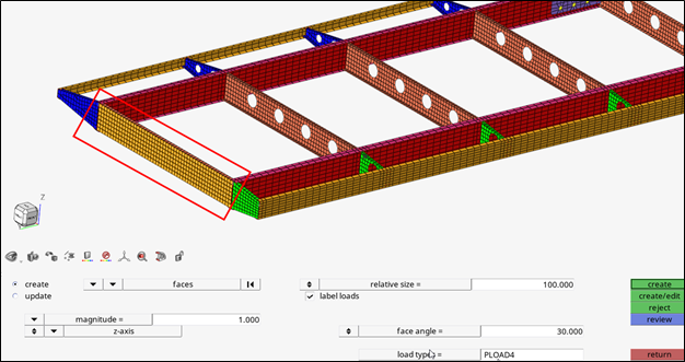
Select faces on the model as shown below.
Figure 6. Faces for Application of Pressure Load at One End of Airframe
Model
For magnitude, enter 1.0.
A pressure load of magnitude 1 MPA is applied.
From the first drop-down menu, change the button from normal to
direction.
In the second drop-down menu, select z-axis as the axis
of application of the pressure load.
For load type=, select PLOAD4.
Click Create.
A force of 1 MPA pressure load is applied to the selected nodes in the
z-direction.
Click return to exit.
Create an SPC Load Collector
In this step, an SPC load collector for constraints is created.
In the Model Browser, select Create > Load Collector.
The Create Load Collector window
opens.
For Name, enter spc.
Click Color and
select a color from the color palette.
For Card Image, select None.
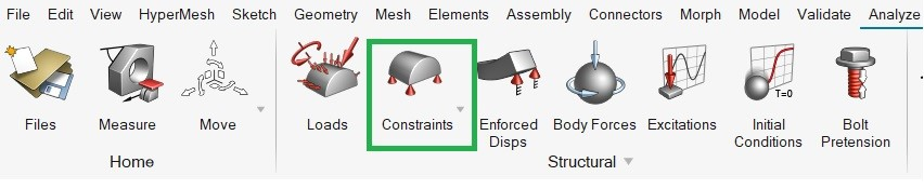
From the menu bar, select the
Analyze ribbon.
From the ribbon, select BCs > Constraints.
Figure 7.
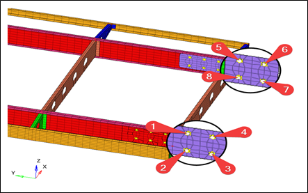
In the panel, select the Create radio button.
Select the nodes on the model as shown below.
Figure 8. Nodes to Constrain the DoFs at One End of Airframe Model
Constrain the nodes in all the degrees of freedom.
Click Create.
Click return to exit.
Create a TLOAD1 Load Step Input
This step creates the transient dynamic response excitation.
In the Model Browser, select Create > Load Step Inputs.
The Create Load Step Inputs window
opens.
For Name, enter TLOAD.
Click Color and
select a color from the color palette.
For Config type, select Dynamic Load - Time Dependent
from the drop-down list.
For Type, select TLOAD1 from the drop-down list.
For Exciteid, click Unspecified and select to open the Advanced Selection
dialog.
Tip: You can also press the Spacebar to open Advanced
Selection.
In the dialog, select Pressure from the list of load
collectors.
Click Apply, then
OK
Similarly, for the TID field select the LOAD_HISTORY
curve to define the time history of the loading.
The type of excitation can be an applied load (force or moment), an enforced
displacement, velocity, or acceleration. The field [TYPE] in the TLOAD1 card
image defines the type of load. The type is set to applied load by
default.
Click Close.
Create Load Step
In this step, a load step for Direct Transient Analysis is created.
In the Model Browser, select Create > Load Step.
The Create Loadstep window opens.
For Name, enter transient.
For Analysis type, select Transient (direct) from the
drop-down menu.
For SPC, click Unspecified and select to open the Advanced Selection
dialog.
Tip: You can also press the Spacebar to open Advanced
Selection.
In the dialog, select spc from the list of load
collectors.
Click OK
Similarly, for the DLOAD field select TLOAD from the
list of load step inputs.
For TSTEP (TIME) select the TIMESTEP load
collector.
Click Close.
A subcase is created that specifies the loads and boundary conditions
for direct transient dynamic analysis.
Create Output Request
In this step, the output request for Transient Dynamic Analysis is created.
On the Analyze ribbon, under the Analyze tool group, select Run > Control Cards.
The Control Cards panel opens.
In the panel, select PARAM.
Select PRGPST from the drop-down menu.
Click No.
Click return.
With this setting, autospc is not printed in the output
file.
On the panel, select GLOBAL_OUTPUT_REQUEST.
Select STRESS.
For FORMAT, select H3D.
For OPTIONS, select ALL.
Click return.
Similarly, select DISPLACEMENT and
SPF and specify the same FORMAT and OPTIONS
settings.
Save the Database
Set the directory in which to save the file.
Click File > Save.
For File name, enter wing_structure.hm.
Click Save.
Run Direct Transient Analysis
From the menu bar, select
Analyze.
On the Analyze ribbon, under the Analyze tool group, select Run
OptiStruct Solver.
The panel area opens.
Click Save as.
For File name, enter wing_structure.fem.
The name and location of the file are displayed in the input file:
field.
Set export options: to all.
Set run options: to analysis.
Set memory options: to memory default.
Click OptiStruct to launch the job.
If the job was successful, new results files appear in the directory
where the OptiStruct model file was written. The
wing_structure.out file is a good place to look for
error messages to help debug the input deck if any errors are present.
The
default files written to the directory are:
wing_structure.html
HTML report of the analysis giving a summary of the problem
formulation and the results.
wing_structure.out
OptiStruct output file containing
specific information on the file setup, the setup of the
problem, estimates for the amount of RAM and disk space required
for the run, and compute time information. Review this file for
warnings and errors that are flagged from processing the
wing_structure.fem file.
wing_structure.h3d
HyperView binary results file.
wing_structure.mvw
HyperView session file. This file is
only created when the transient analysis is performed. This file
automatically creates plots for the displacement, velocity, and
acceleration results contained in the file.
wing_structure.stat
Summary of the analysis process, providing CPU information for
each step during the analysis process.
Post-Process the Results
In this step, the wing structure results are reviewed in HyperMesh.
In HyperMeshmenu bar, select Post.
On the Post ribbon, select Results.
Figure 9.
From the Results Browser, right-click the last timestep in
the results and select Make Current from the context menu.
On the Post ribbon, select Contour.
Figure 10.
In the Contour window, for Data type select
Displacement.
For Component, select Z-direction.
In the modeling window, select all components.
Close the Contour window and select to plot
the result.
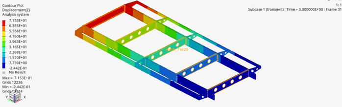
Figure 11. Displacement in Z Direction of Wing Structure for Direct Transient
Dynamic Analysis
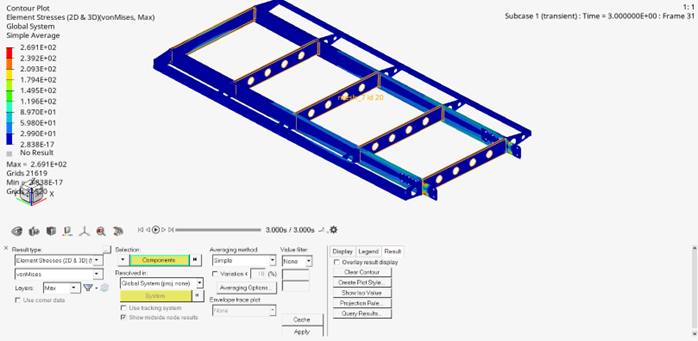
Similarly, plot the results for Von Mises element stresses (2D &
3D).
Figure 12. Elemental Stresses in Simple Average of Wing Structure for Direct
Transient Dynamic Analysis


 to add a curve.

 to open the Advanced Selection
dialog.
Tip: You can also press the Spacebar to open Advanced Selection.
to open the Advanced Selection
dialog.
Tip: You can also press the Spacebar to open Advanced Selection. .
The panel area opens.
.
The panel area opens.

 to plot
the result.
to plot
the result.