HL-T: 1040 Factor of Safety (FOS)
Tutorial Level: Beginner
In this tutorial you will:
- Import a model to HyperLife
- Select the FOS module and define its required parameters
- Create and assign materials
- Assign load histories for scaling the stresses from FEA subcases
- Evaluate and view results
Before you begin, copy the file(s) used in this tutorial to your
working directory.
Import the Model
-
From the Home tools, Files tool group, click the Open Model tool.
Figure 1. 
-
From the Load model and result dialog, browse and select
HL-1040\Springlink_FOS.h3d for the model
file.
The Load Result field is automatically populated. For this tutorial, the same file is used for both the model and the result.
-
Click Apply.
Figure 2. 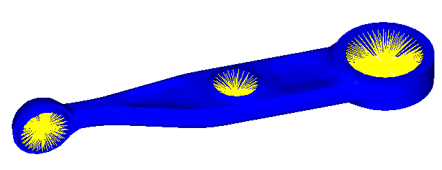
Tip: Quickly import the model by dragging and
dropping the .h3d file from
a windows browser into the HyperLife
modeling window.
Define the Fatigue Module
-
Click the arrow next to the fatigue module icon and select the
FOS tool from the list of options.
Figure 3. 
The FOS dialog opens. -
Accept the default parameters.
Figure 4. 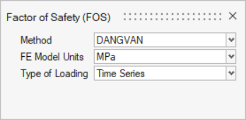
- Exit the dialog.
Assign Materials
-
Click the Material tool.
Figure 5. 
The Assign Material dialog opens. - Activate the checkbox for the part spring_link_fine.
-
Edit the FOS material.
- Click the My Material tab.
- Enter a value of 1000 for TFL.
- Enter a value of 0.5 for HSS.
- Enter a value of 0.0 for Shear Threshold.
- Enter a value of 0.0 for Safe Zone Angle.
- Click Plot and Save.
Figure 6. 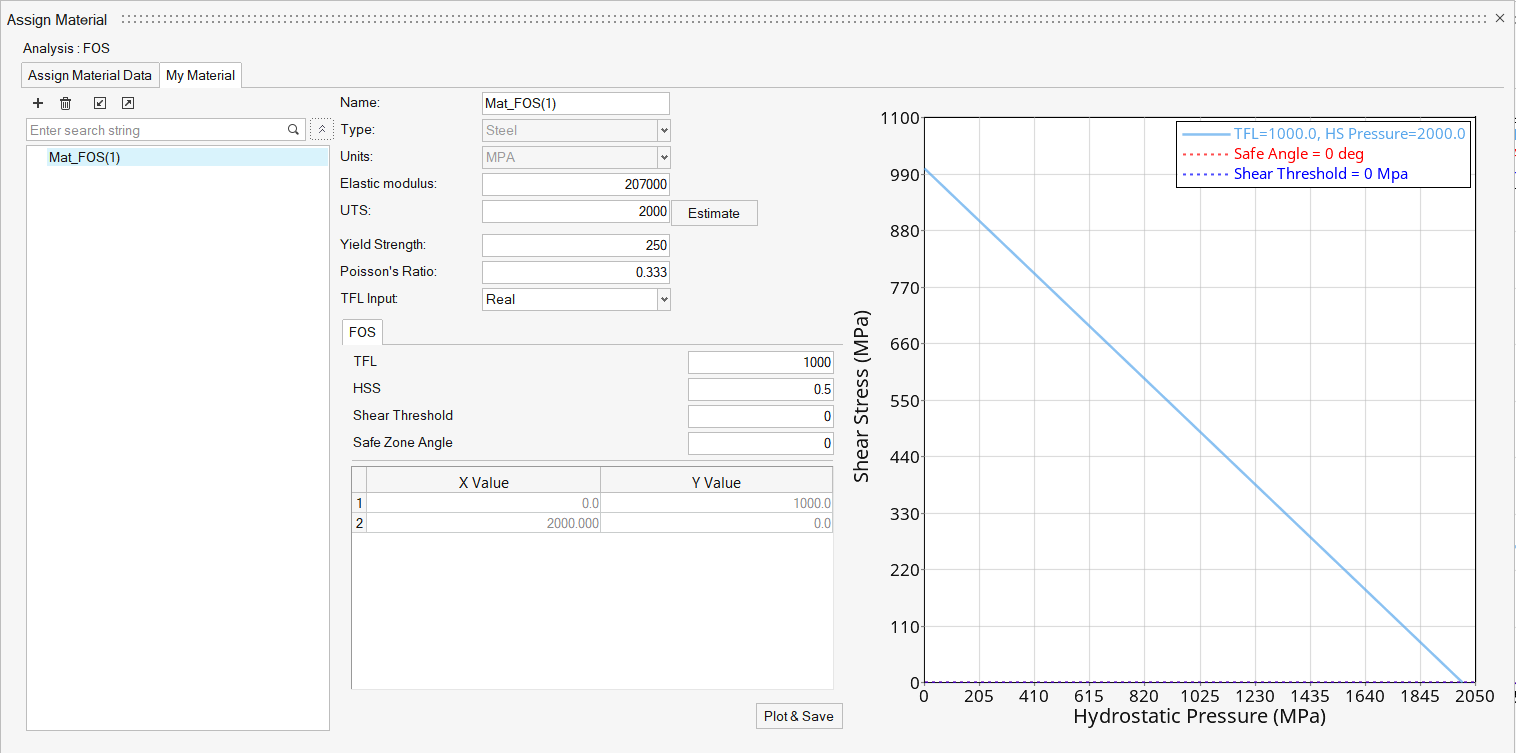
- Click the Assign Material Data tab.
-
Verify the following properties.
Figure 7. 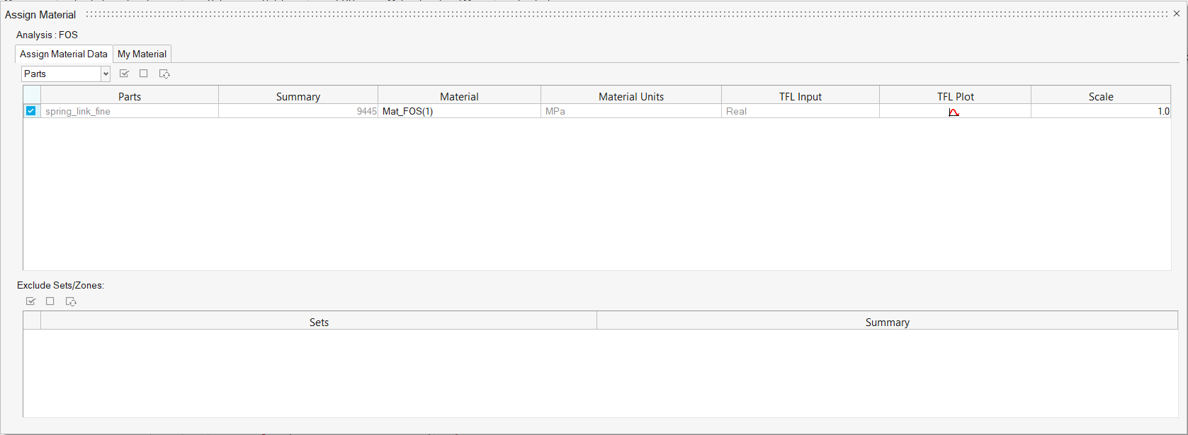
- Exit the dialog.
Assign Load Histories
-
Click the Load Map tool.
Figure 8. 
The Load Map dialog opens. - From the Channel Type drop-down menu at the top of the dialog, select Time Data.
-
Click
 in the Choose File
field and browse for load1.csv.
in the Choose File
field and browse for load1.csv.
-
Click
 to add the load case.
- Optional:
Click
 to view a plot of the load.
Figure 9. Load 1 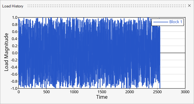
Tip: Expand the width of the dialog to view a clearer picture of the plot. -
On the bottom half of the dialog, set the radio button to
Manual for event creation and click three times to create three event headers.
- Drag and drop Subcase 1 under Event_1, Subcase 2 under Event_2, and Subcase 3 under Event_3.
- Drag and drop the Block file under load1 onto the Channels field of all three subcases.
- Activate the checkboxes for the three events.
- Set LDM to 1.0, Scale to 3.0 and Offset to 0.0 for Subcase 1.
-
Right-click on the Scale field of Subcase 1 and select Apply value
to all events.
Figure 10. 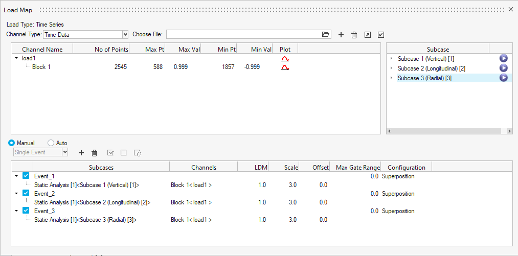
- Exit the dialog.
Evaluate and View Results
-
From the Evaluate tool group, click the
Run Analysis tool.
Figure 11. 
The Evaluate dialog opens.Figure 12. 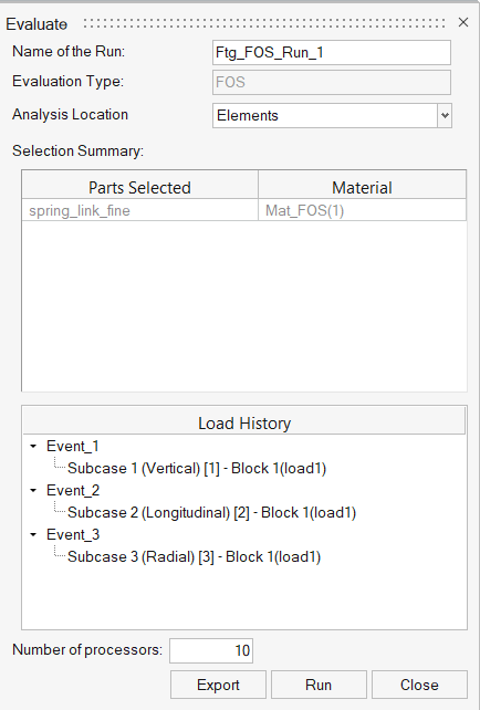
- Optional: Enter a name for the run.
-
Click Run.
Result files are saved to the home directory and the Run Status dialog opens.
- Once the run is complete, click View Current Results.
-
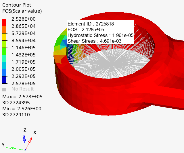
Use the Results Explorer to
visualize various types of results.
Figure 13.