HL-T: 1000 Uniaxial Stress-Life (S-N)
Tutorial Level: Beginner
In this tutorial you will:
- Import a model to HyperLife.
- Select the SN module and define its required parameters.
- Assign materials.
- Assign load histories for scaling the stresses from FEA subcases.
- Evaluate and view results.
Import the Model
-
From the Home tools, Files tool group, click the Open Model tool.
Figure 1. 
-
From the Load model and result dialog, browse and select
HL-1000\Shaft.h3d for the model
file.
The Load Result field is automatically populated. For this tutorial, the same file is used for both the model and the result.
-
Click Apply.
Figure 2. 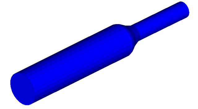
Tip: Quickly import the model by dragging and
dropping the .h3d file from
a windows browser into the HyperLife
modeling window.
Define the Fatigue Module
-
Click the SN tool.
The SN tool should be the default fatigue module selected. If it is not, click the arrow next to the fatigue module icon to display a list of available options.
Figure 3. 
The SN dialog opens. -
Define the SN configuration parameters.
- Select Uni Axial as the method.
- Select MPa for the FE model units.
- Select Signed von for the stress combination.
- Enter a value of 0.5 for the certainty of survival.
- Select GOODMAN for the mean stress connection.
- Select Worst for the layer selection.
- Select Time Series for the type of loading.
Figure 4. 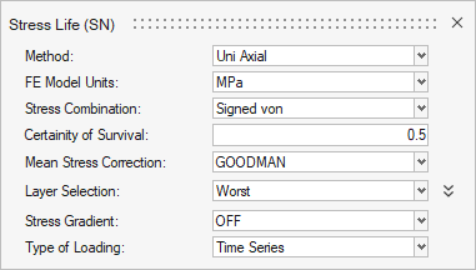
- Exit the dialog.
Assign Materials
-
Click the Material tool.
Figure 5. 
The Assign Material dialog opens. - Activate the checkbox next to the part solid.
-
If Steel 1045, Annealed, BHN=225 (932) is not the default material assigned to
the part:
-
Right-click on Steel 1045, Annealed, BHN=225
(932) and select Add to Assign Material
List.
Figure 6. 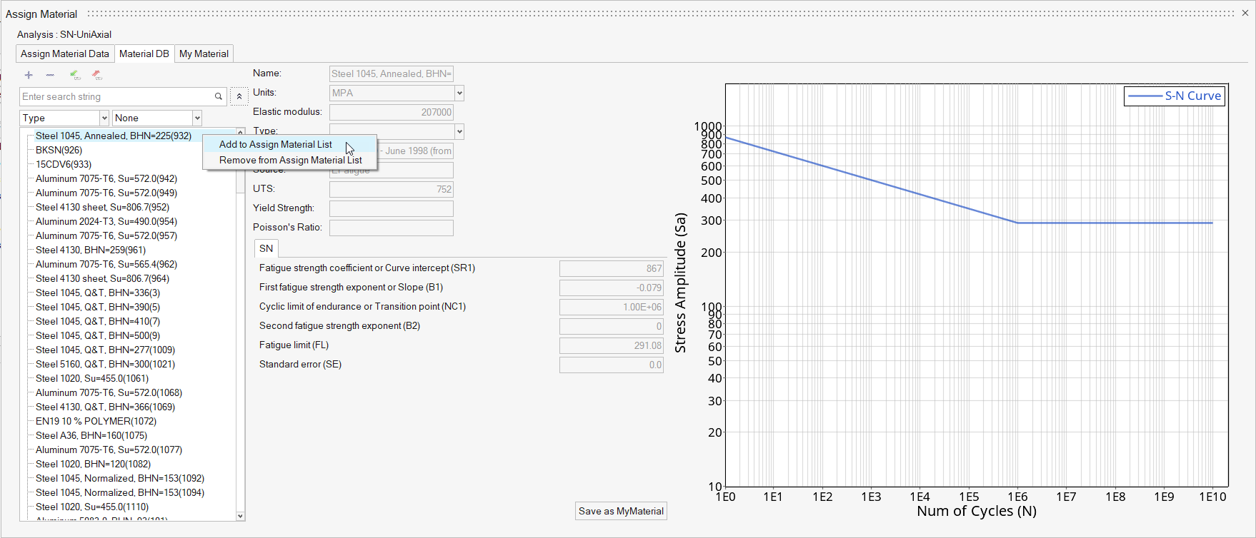
-
Right-click on Steel 1045, Annealed, BHN=225
(932) and select Add to Assign Material
List.
- Optional:
Click
 to
review the SN plot.
to
review the SN plot.
Figure 7. 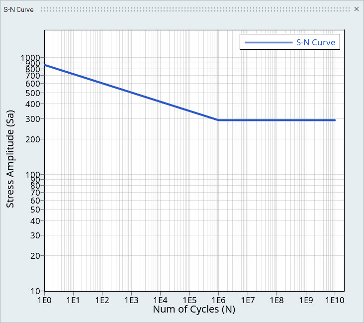
-
Accept all other default parameters.
Figure 8. 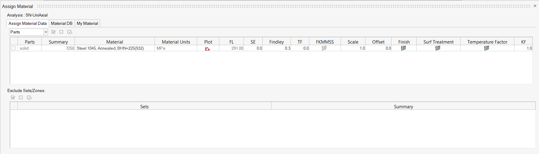
Note: The FL (Fatigue Limit) and SE (Standard Error) values are from the SN curve selected for the part. The SE value can be edited from both the Assign Material Data tab and the My Material tab. The FL value can be reviewed and edited from the My Material tab. Parameters updated in the My Material tab will be saved to a user-defined excel spreadsheet. - Exit the dialog.
Assign Load Histories
-
Click the Load Map tool.
Figure 9. 
The Load Map dialog opens. - From the Channel Type drop-down menu at the top of the dialog, select Time Data.
-
Click
 in the Choose File
field and browse for load1.csv.
in the Choose File
field and browse for load1.csv.
-
Click
 to add the load case.
- Repeat steps 3 and 4 for load2.csv.
- Optional:
Click to view a plot of the loads.
Figure 10. Load 1 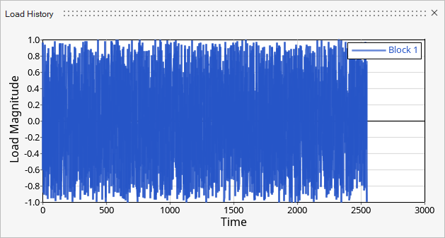
Figure 11. Load 2 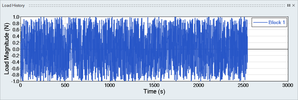
Tip: Expand the width of the dialog to view a clearer picture of the plot. -
On the bottom half of the dialog, set the radio button to
Manual for event creation and click to create an
Event_1 header.
- Drag and drop Subcase 1 and Subcase 2 under Event_1.
- Drag and drop the Block file under load1 onto the Channels field of Subcase 1.
- Repeat for the Block file under load2 and Subcase 2.
- Activate the Event_1 checkbox.
-
Set LDM to 1.0, Scale to 5.0 and
Offset to 0.0 for both subcases.
Figure 12. 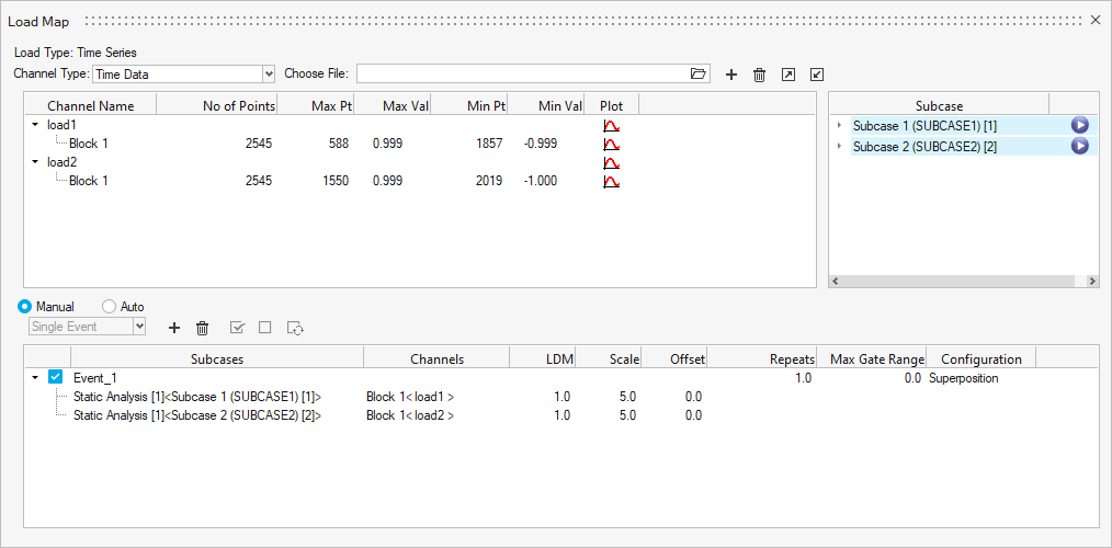
- Exit the dialog.
Evaluate and View Results
-
From the Evaluate tool group, click the
Run Analysis tool.
Figure 13. 
The Evaluate dialog opens.Figure 14. 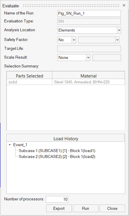
- Optional: Enter a name for the run.
-
Click Run.
Result files are saved to the home directory and the Run Status dialog opens.
- Once the run is complete, click View Current Results.
-
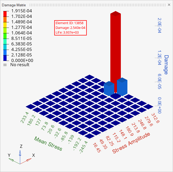
Use the Results Explorer to
visualize various types of results.
Figure 15. 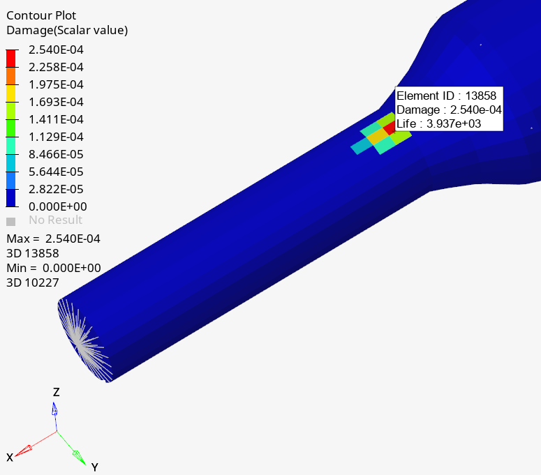
Figure 16.