The fitting process begins with an optimization run. The goal of this optimization is
to obtain a reasonable set of starting values for the design parameters.
The fitting tool uses the parameters defined in the initial
.gbs file, and then attempts to refine these values
using a method known as single-point fitting.
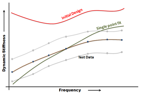
The objective of single-point fitting is to select a single point in the
middle of the data, and then fit the parameters to that selected point. The
parameters are used to compute the cost function, Cost (b), for all
frequencies and amplitudes.
If the cost is less than the cost calculated with the original design, the
new design is accepted as the starting point.
If the cost is greater than the cost computed with the original design, an
adjacent point is selected and the single point fitting is repeated.
This operation continues until a better initial design is found. In the
unlikely scenario that no single point fit is better than the original
design, the original design is used as the starting point.
Single point fitting is very fast and the optimizer converges in just a few
iterations. The following plot shows the effect of a single point fit:Figure 1.