The Riemann problem can be defined as a category of initial value problems that
involve a conservation equation and a piecewise data set with a single
discontinuity.
In terms of SPH, you can solve a Riemann problem for each pair of particles, yielding
a more isotropic particle distribution and smoother gradients in the solution. The
following depiction is based on the work of C.
Zhang. Given the Riemann problem definition, you start off by
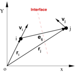
constructing a unit vector between two particles and . The two particles can then be assumed to be the
left and right sides of the Riemann problem, such that the physical values of
density (), velocity () and pressure () are expressed as:
Where, is the velocity vector of the respective particle,
which is illustrated in Figure 1. C.
ZhangFigure 1. Construction of the Riemann problem in SPH
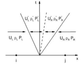
The discontinuity is assumed to be located at the interface (Figure 1), half
way between the particles. Assuming that particles are moving with arbitrary
velocity vectors, the consequent solution of their motion is either a rarefaction or
compression wave. However, there is a third wave solution at the interface denoted
with * exponent, where and , as indicated by the dashed link in Figure 2.Figure 2. Simplified Riemann Problem Solution in Time. This example shows three possible waves.C.
Zhang
From these basic assumptions, you can derive the and values as:
Where, the index denotes the mean value of the respective value
between the two particles.
With these two solutions to the Riemann problem, you can modify the continuity
equation and the pressure gradient term in the momentum equation as
follows:
Where, .
It is well-known that 1st order Riemann solvers such as the one illustrated here are
dissipative. To that extent, nanoFluidX is using a limiter so that
the Riemann solutions are provided only when the fluid is under compression. This
effectively reduces the dissipation and has been shown to improve the results in
various situations. C.
Zhang
Note: Although the Riemann solver option is experimental,
canonical test cases, simple geometries, and problems involving single phase
runs such as tank sloshing or water management should still greatly benefit from
the new formulation. However, industrial gearboxes and violent multiphase flows
in complex moving geometries in general are likely to experience local
instabilities. This will be addressed in the coming versions of nanoFluidX.
Density filtering is an integral part of the Riemann solver implementation. In SPH
simulation, the consistency between mass, density, and occupied area cannot be
strictly enforced. Several density filtering schemes have been developed to tackle
this. In nanoFluidX, two versions are implemented:
INCREMENTAL and INSTANT filtering.
INSTANT
The instant density filtering is basically a 0th-order Shepard filter.
At each evaluation point (according to the number set by
RM_freq_rho_init), the density is re-calculated
by:
Where,
Density of particle I
Mass of particle j
Volume of particle j
Weight calculated from the kernel function
INCREMENTAL
A modified 1st-order density filtering scheme is used as an additional
option. The operator is calculated following:
Where, is the density from solving the
continuity equation before applying the filter.