The Performance mapping / Efficiency map
The Performance mapping / Efficiency map for evaluating the performance of the wound field synchronous machines.
Positioning and objective
The aim of the test “Performance mapping – Sine wave – Motor – Efficiency map” is to characterize the behavior of the machine in the "Torque-Speed" area.
Input parameters like the maximum “Field current”, the maximum “Line current”, maximum “Line-Line voltage”, and the desired “Maximum speed” of the machine are considered.
Only the Maximum Torque Per Volt command mode (MTPV) is available in this version. The Maximum Torque Per Amps command mode (MTPA) will be provided in the next releases.
Input parameters define the torque-speed area in which the evaluation of the machine’s behavior is performed.
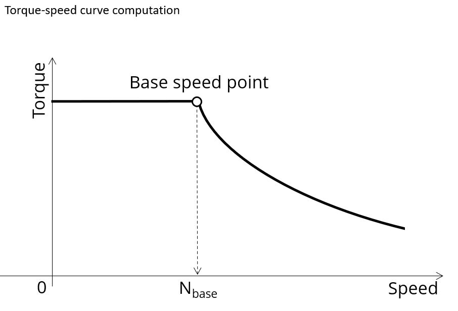 |
| Characterization of the corner point on the torque-speed curve |
Here is an overview of the test, given below.
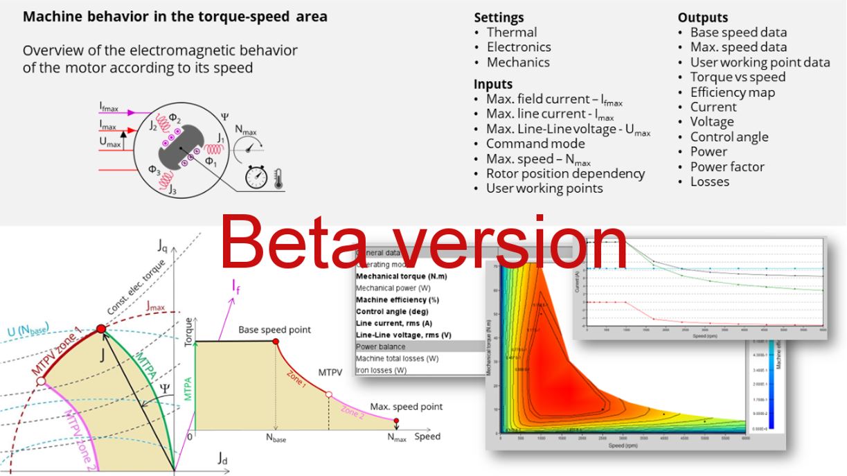 |
| Performance mapping / Efficiency map – Synchronous Machines with wound field – Inner salient pole - Inner rotor (SMWF-ISP-IR) - Overview |
User inputs
The main user input parameters needed to perform this test are the maximum allowed supplied, field current, line current, line-line voltage, the targeted maximum speed, and the command mode. Winding temperatures must also be set.
When required, the location of the working points (single point or duty cycle) to be evaluated must be defined as inputs.
Four advanced user input parameters allow adjusting the compromise between accuracy and computation time: the number of computations for Jd-Jq, the number of computations for If, for speed, and for torque.
Please see additional information in the section below (the import button allows sharing the data simulated in Flux between model map and efficiency tests).
Main outputs
Different kinds of outputs are displayed, like data, curves, maps, and tables.
In the results, the performance of the machine at the base point (the base speed point) and for the maximum speed set by the user are presented. A set of curves (like Torque-Speed curve) and maps (like Efficiency map) are computed and displayed.
Here are below illustrations of some results that can be provided in the test.
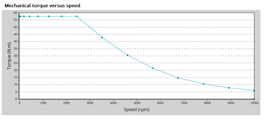 |
| Mechanical torque versus speed - Example |
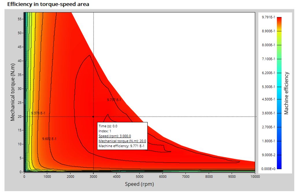
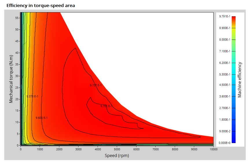 |
| Efficiency in torque-speed area - Example |
 |
| A “single” working point displayed on the efficiency map - Example |
The second feature allows the user to define a duty cycle by giving a list of working points (speed, torque) versus time. The displayed results illustrate the machine performance over the considered duty cycle (mean, min, and max values).
The time variation of the main quantities is also displayed (mechanical torque, speed, control angle, current, voltage, power, efficiency, and losses).
All the corresponding points are displayed on the different map provided. Each working point can be selected to visualize the corresponding main information.
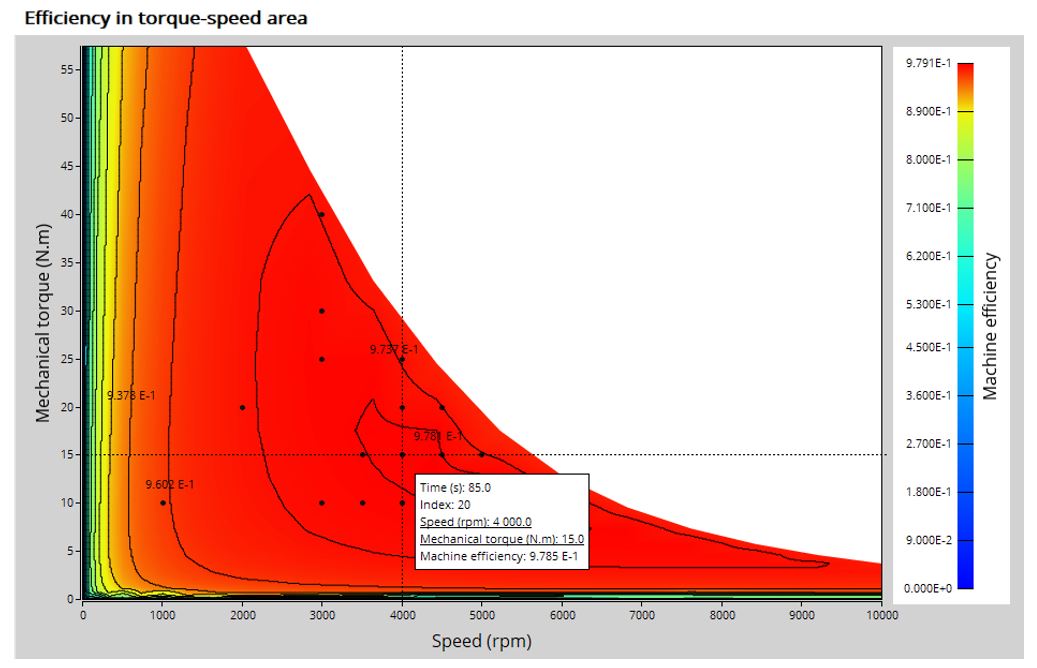 |
| A “Duty cycle” displayed on the efficiency map - Example |
- Machine performance - Base speed point
- Machine performance - Maximum speed
- Machine performance - User working point (when requested)
- Machine performance - Duty cycle analysis (when requested)
- Power electronics (when requested by the user)
- Torque-speed curves and maps
- Efficiency in torque-speed area
- Current (If, J, Jd, Jq) in torque-speed area
- Voltage (Vf, V, Vd, Vq) in torque-speed area
- Control angle in torque-speed area
- Power in the torque-speed area (machine electrical power, stator electrical power, excitation power, mechanical power, system electrical power) in the torque-speed plane
- Power factor in torque-speed area
- Losses in the torque-speed area (total, Joule, iron, mechanical, power electronics, and additional) in the torque-speed plane
- Duty cycle curves (when requested)
In the results, the performance of the machine at the base point (base speed point) and for the maximum speed set by the user are presented.
A set of curves (like Torque-Speed curve) and maps (like Efficiency map) are computed and displayed.
Main principles of computation
- Raw data and Park’s model
- Identification of the torque-speed curves and maps
Raw data and Park’s model
The first step consists of computing the raw data that characterizes the machine in the three dimensions If - Jd - Jq. This is done using Finite Element modelling (Flux® – Magnetostatic application).
To do that, a grid of values (Jd, Jq) is considered for all levels of If.
For each node of this grid, the corresponding flux linkage through each phase is extracted (a, b, c). Fux density in regions (teeth and yoke of the machine) is also extracted.
 |
| Raw data – Test “Performance mapping – Sine Wave – Motor – Efficiency map” |
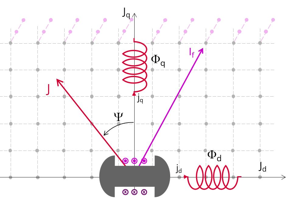
The second step consists of using the raw data with Park’s model.
D-axis flux-linkage component (d) and Q-axis flux-linkage component (q) are computed according to the Park’s transformation.
The Electromagnetic torque Tem is computed in different ways as a function of the input rotor position dependency value.
If rotor position dependency is set to “No”, the flux linkage maps, and the following formula are used:
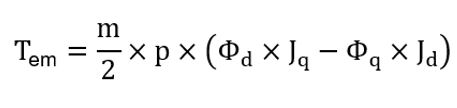
Where m is the number of phases (3) and p is the number of pole pairs. Jd and Jq are the d and q axis peak current.
Identification process for the torque-speed curves and maps
Below are the three main steps involved in building the efficiency map and other associated results.
- Building of the torque-speed curve and other associated results
- Define the grid in the area under the torque-speed curve
- Building of the efficiency map and other associated results
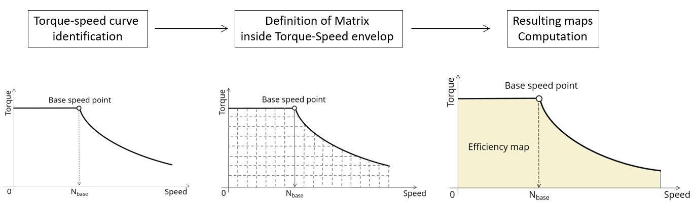 |
| Main steps of the computation algorithm |
For more information, refer to MotorFactory_2024_ SMWF_ISP_IR_3PH_Test_PerformanceMapping.pdf
The import button allows sharing the data simulated in Flux between model map and efficiency tests.
By implementing the rotor position dependency option for the model map test and efficiency map test of synchronous machines, this update facilitates the seamless transfer of settings, inputs, and crucially, simulated data in Flux between the two tests. As they use the same Flux data in most cases and significant computation time is required to obtain it, users can now accelerate the test resolution and optimize their workflow.
- Reluctance Synchronous Machines - Inner rotor
- Synchronous Machines with wound field – Inner Salient Pole - Inner rotor
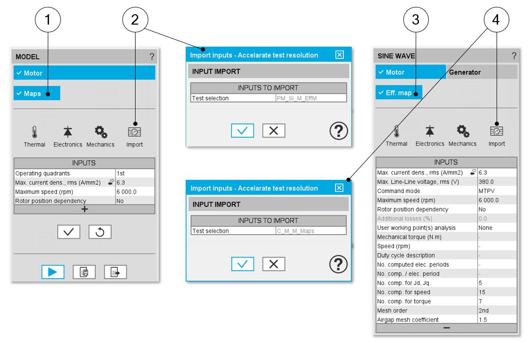
Upon completing a model map test, users can activate the import button in the efficiency map test GUI. This enables them to effortlessly import the settings and corresponding Flux data from the previous test, eliminating the need to rerun Flux for identical data, a step that typically consumes a substantial portion of computation time during efficiency mapping.
 |
|
| Import function in Model Map test and Efficiency Map test to accelerate test resolution | |
| 1 | Open model map test environment when an efficiency map test is available for import |
| 2 | Click the import button and import the settings, inputs, and Flux data of the latest efficiency map test |
| 3 | Open efficiency map test environment when a model map test is available for import |
| 4 | Click the import button and import the settings, inputs, and Flux data of the latest model map test |