Inputs
Introduction
The total number of user inputs is equal to 11.
Among these inputs, 4 are standard and 7 are advanced inputs.
Standard inputs
- Maximum Line-Line voltage, rmsThe rms value of the maximum Line-Line voltage supplying the machine: “Maximum Line-Line voltage, rms” (Maximum Line-Line voltage, rms value) must be provided.Note: The number of parallel paths and the winding connection are automatically considered in the results.
- Rated power supply frequency
The value of the rated power supply frequency of the machine: “Rated power supply frequency” (rated power supply frequency) must be provided.
The rated power supply frequency is the electrical frequency applied at the terminals of the machine for the base speed point.
- Maximum speed
The value of the « Maximum speed » (Maximum speed).) must be provided.
The analysis of the test results is performed over a given speed range defined between 0 and the maximum speed. This allows to evaluate the behavior of the machine as a function of speed (like rotor Joule losses, total losses, power factor...) in this range of speed.
Advanced inputs
- Electrical equivalent scheme identification
In the first step of the internal process of computation, it is required to identify the model (non-linear electrical equivalent scheme). This implies the computation for each component of the electrical scheme (resistance and inductances maps) as a function of the Line-Line voltage and the power supply frequency.
Both following inputs allow to fix the discretization required to identify the non-linear model.
- Model maps identification - Number of computations for Line-Line
voltage
The number of computations for the voltage must be defined with the user input « ID - No. Comp. for voltage » (Electrical equivalent scheme identification - Number of computations for Line-Line voltage).
The default value is equal to 10. This default value provides a good tradeoff between the accuracy and the computation time. The minimum allowed value is 10.Note: We recommend increasing « ID - No. Comp. for voltage » to at least to 15 in case of fractional slot per pole and per phase. - Model maps identification - Number of computations for power supply
frequency
The number of computations for the frequency must be defined with the user input « ID - No. Comp. for freq. » (Electrical equivalent scheme identification - Number of computations for power supply frequency).
The default value is equal to 10. This default value provides a good tradeoff between the accuracy and the computation time. The minimum allowed value is 10Note: We recommend increasing « ID - No. Comp. for freq. » at least to 15 in case of fractional slot per pole and per phase.. -
Operation of the non-linear model to generate
T(U,f,s)
In the second step of the internal process of computation, it is required to operate (solve) the model (non-linear electrical equivalent scheme) to generate sets of curves in function of the Line-Line voltage, the power supply frequency, and the slip to get the performances of the machine as in the T(Slip) test.
Forth following inputs allow to fix the discretization required to operate the non-linear model in order to get the data set of T(U,f,s) curves representing the behavior of the machine in function of the Line-Line voltage, the power supply frequency and the slip(or speed).
- Operation of model to generate T(U,f,s) - Number of computations for
Line-Line voltage
The number of computations for the voltage must be defined with the user input « OP. - No. comp. for voltage » (Operation of model to generate T(U,f,s) - Number of computations for Line-Line voltage).
The default value is equal to 20. This default value provides a good overview of the machine behavior. The minimum allowed value is 10.Note: The computation time of the test is not highly impacted by this input and huge values can be used as in the test Scalar EM in which the default value is 300. - Operation of model to generate T(U,f,s) - Number of computations for power
supply frequency
The number of computations for the frequency must be defined with the user input « Op. - No. comp. for freq. » (Operation of model to generate T(U,f,s) - Number of computations for power supply frequency).
The default value is equal to 30. This default value provides a good overview of the machine behavior. The minimum allowed value is 10.Note: The computation time of the test is not highly impacted by this input, and huge values can be used as in the test Scalar EM in which the default value is 500. - Operation of model to generate T(U,f,s) – Slip distribution modeThe computation of the test « Characterization – Model – Motor – Scalar » is performed by considering a distribution of computed points. The user’s input “Slip distribution mode” (Select the method for the distribution of computed points) gives three possibilities to the user:
- Slip distribution mode = Logarithmic
When “Logarithmic” is selected, the distribution of the computed points is automatically done. The number of computations to be done in the slip range must be set in the next field: “No. comp. in slip range”.
- Slip distribution mode = Linear
When “Linear” is selected, the distribution of the computed points is automatically done. The number of computations to be done in the slip range must be set in the next field: “No. comp. in slip range”.
- Slip distribution mode = Table
When “Table” is selected, the list of slips to be considered must be defined by using the next field: “Slip table” and by clicking on the button “Set values”.
Two ways are possible to fill the table: either filling the table line by line or by importing an excel file where all the slips to be considered are defined.Note: The slips must be listed in ascending order.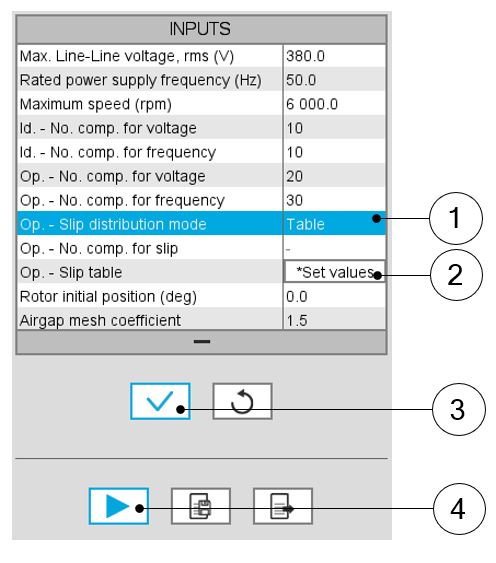
Slip distribution mode = Table 1 Select the “Table” option. 2 Click the button “Set values” of the field “Slip table” to open a dialog box to define the list of slips to be considered.
Refer to the next illustration which shows how to fill the Slip table.
3 Button to validate and consider the user inputs 4 Button to run the computation 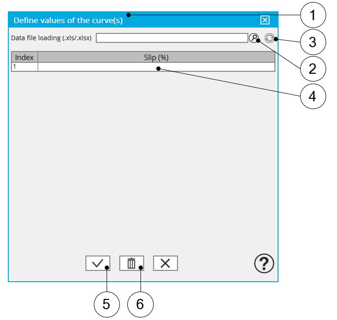
Slip distribution mode = Table – Dialog box to define the list of slips 1 Dialog box opened when clicked on the button “Set values” in the field “Slip table” 2 Browse the folder to select an Excel file which defined the list of slips 3 Button to refresh the table data when the considered Excel file has been modified 4 Fields to be filled with data to describe the considered slips 5 Button to apply the inputs 6 Button to erase the data table Note: The Excel template used to import a list of slips is stored in the folder Resource/Template in the installation folder of FluxMotor®. An example of this template is displayed below.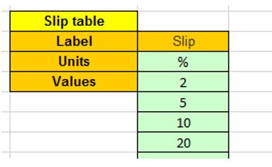
Excel file template to define the list of slips Note: The slips must be listed in ascending order, and we recommend defining at least a hundred values. - Operation of model to generate T(U,f,s) - Number of computations
for slip
The number of computations for the slip must be defined with the user input « Op. - No. comp. for slip » (Operation of model to generate T(U,f,s) - Number of computations for slip).
The default value is equal to 100. This default value provides a good overview of the machine behavior. The minimum allowed value is 10.Note:- The machine operating mode is “Motor”, so the slip range is [0,1].
- The slip distribution mode used is logarithmic or linear.
- The computation time of the test is not highly impacted by this input and huge values can be used if needed as 200.
- Operation of model to generate T(U,f,s) – Slip tableWhen the choice of point distribution mode is “Table”, the list of slips to be considered “Op. - Slip table” (Operation of model to generate T(U,f,s) - Slip table) must be provided. Refer to the above section 2) Slip distribution mode = TableNote: The machine operating mode is fixed to“Motor”, so the slip range is ]0,1].
- Skew model – No. of layers
When the rotor bars or the stator slots are skewed, the number of layers used in Flux® Skew environment to model the machine can be modified: “Skew model - No. of layers” (Number of layers for modelling the skewing in Flux® Skew environment).
- Rotor initial position
The initial position of the rotor considered for computation can be set by the user in the field « Rotor initial position » (Rotor initial position). The default value is equal to 0.
The range of possible values is [-360, 360].Note: The rotor initial position has an impact only on the induction curve in the air gap. - Airgap mesh coefficient
The advanced user input “Airgap mesh coefficient” is a coefficient which adjusts the size of mesh elements inside the airgap. When the value of “Airgap mesh coefficient” decreases, the mesh elements get smaller, leading to a higher mesh density inside the airgap, increasing the computation accuracy.
The imposed Mesh Point (size of mesh elements touching points of the geometry), inside the Flux® software, is described as:
Mesh Point = (airgap) x (airgap mesh coefficient)
Airgap mesh coefficient is set to 1.5 by default.
The variation range of values for this parameter is [0.05; 2].
0.05 gives a very high mesh density and 2 gives a very coarse mesh density.CAUTION: Be aware, a very high mesh density does not always mean a better result quality. However, this always leads to a huge number of nodes in the corresponding finite element model. So, it means a need of huge numerical memory and increases the computation time considerably.
- Slip distribution mode = Logarithmic